

Warren Buffett & Put Selling
How Risk-Neutral Distributions Differ from Real-World Distributions

While Warren Buffett is undeniably one of the most successful investors in history, the reasoning he gave supporting his decision to sell put options in the years prior to the 2008 financial crisis suggests that expertise in one area of finance doesn't necessarily translate to all areas. Buffett's Berkshire Hathaway sold billions of dollars worth of long-dated put options on various market indexes, essentially betting that markets would be higher when the options expired. While this strategy ultimately proved profitable due to the market's long-term recovery, it exposed Berkshire to significant mark-to-market losses in the short term. In this post, we discuss why the reasons that Buffett gave for selling puts were wrong, and why it worked out for him in the end anyways.
Berkshire Hathaway’s Puts
Put options allow the put buyer to sell the underlying asset to the put seller at an agreed date (expiration) and price (strike). One can think of them as a sort of insurance: an investor owning SPY but fearing a market crash can buy a put that gives them the right to sell the ETF at a predetermined strike price. Initially this seems like a sound hedge, but many investors balk once they see the put’s premium. On the put seller’s side, shorting a put profits when the underlying rises and loses when it falls.
Some readers may wonder why not simply use a stop order. That’s fair, but execution often incurs costs—especially in turbulent markets (imagine CalPERS triggering a $50 B stop order during the financial crisis). Efficient markets ensure hedging execution costs are priced into derivatives, so we’ll return to that later.
In the years before the financial crisis, Warren Buffett wrote long-dated, deep-out-of-the-money puts. In his 2008 Annual Letter he described those positions:
“I believe each contract we own was mispriced at inception, sometimes dramatically so… We have added modestly to the ‘equity put’ portfolio I described in last year’s report. Some of our contracts come due in 15 years, others in 20. We must make a payment to our counterparty at maturity if the reference index to which the put is tied is then below what it was at the inception of the contract. Neither party can elect to settle early; it’s only the price on the final day that counts… Our put contracts total $37.1 billion (at current exchange rates) and are spread among four major indices: the S&P 500 in the U.S., the FTSE 100 in the U.K., the Euro Stoxx 50 in Europe, and the Nikkei 225 in Japan. Our first contract comes due on September 9, 2019 and our last on January 24, 2028.”
Buffett believed these puts exploited mis-specifications of the Black-Scholes model. He illustrated with a 100-year put example:
“If the [Black-Scholes option pricing] formula is applied to extended time periods, however, it can produce absurd results… Suppose we sell a 100-year $1 billion put option on the S&P 500 at a strike price of 903 (the index’s level on 12/31/08). Using the implied volatility assumption for long-dated contracts that we do, and combining that with appropriate interest and dividend assumptions, we would find the ‘proper’ Black-Scholes premium for this contract to be $2.5 million.
To judge the rationality of that premium, we need to assess whether the S&P will be valued a century from now at less than today. Certainly the dollar will then be worth a small fraction of its present value (at only 2% inflation it will be worth roughly 14¢). So that will be a factor pushing the stated value of the index higher. Far more important, however, is that one hundred years of retained earnings will hugely increase the value of most of the companies in the index. In the 20th Century, the Dow-Jones Industrial Average increased by about 175-fold, mainly because of this retained-earnings factor.
Considering everything, I believe the probability of a decline in the index over a one-hundred-year period to be far less than 1%. But let’s use that figure and also assume that the most likely decline—should one occur—is 50%. Under these assumptions, the mathematical expectation of loss on our contract would be $5 million ($1 billion × 1% × 50%). But if we had received our theoretical premium of $2.5 million up front, we would have only had to invest it at 0.7% compounded annually to cover this loss expectancy. Everything earned above that would have been profit. Would you like to borrow money for 100 years at a 0.7% rate?
Let’s look at my example from a worst-case standpoint. Remember that 99% of the time we would pay nothing if my assumptions are correct. But even in the worst case among the remaining 1% of possibilities—that is, one assuming a total loss of $1 billion—our borrowing cost would come to only 6.2%. Clearly, either my assumptions are crazy or the formula is inappropriate.
The ridiculous premium that Black-Scholes dictates in my extreme example is caused by the inclusion of volatility in the formula and by the fact that volatility is determined by how much stocks have moved around in some past period of days, months or years. This metric is simply irrelevant in estimating the probability-weighted range of values of American business 100 years from now. (Imagine, if you will, getting a quote every day on a farm from a manic-depressive neighbor and then using the volatility calculated from these changing quotes as an important ingredient in an equation that predicts a probability-weighted range of values for the farm a century from now.)
Though historical volatility is a useful—but far from foolproof—concept in valuing short-term options, its utility diminishes rapidly as the duration of the option lengthens. In my opinion, the valuations that the Black-Scholes formula now place on our long-term put options overstate our liability.”
The introduction to this post clearly suggests I think Buffett is wrong. The technical explanation that follows shows that by selling puts—positions that lose when stocks fall and gain when stocks rise—Buffett gave himself leveraged equity exposure. Moreover, his counterparty, via delta-hedging, could still earn a low-risk profit net of execution costs, provided the implied volatility paid was below the market’s realized volatility over the options’ lifespan. This mirrors how an investor borrowing to take leveraged equity exposure—and their lender—can both profit when the equity premium exceeds their financing cost.
Delta Hedging & Volatility Arbitrage
To people not familiar with options pricing, it usually comes as a surprise to learn that an option’s value is largely independent of the expected returns of the underlying. It is natural to think that a call option (the right but not the obligation to buy the underlying at a future expiry at an agreed-upon strike) should be worth more if the underlying has higher expected returns.
However, the directional exposure of an options position can be removed via delta hedging. The core idea is that since the price of an option is a function of (among many variables) the price of the underlying, then a position in the underlying equal to the negative of the partial derivative of the option value with respect to the underlying (i.e. the “delta” of the option) will reduce the combined position’s net exposure to the underlying to a negligible amount for small moves. As the underlying moves, the trader continuously adjusts his position in the underlying asset to offset the changing exposure of the option. For example, a delta of 0.5 means that for every $1 change in the underlying asset’s price, the option’s price is expected to change by $0.50. By shorting 50 shares of the underlying for each options contract (options are traded with a 100× multiplier), our net position has almost no exposure to small moves in the underlying.
As the underlying moves, we need to either increase or decrease our holding of the underlying since the delta of the option keeps changing (a deep in-the-money option clearly has a higher delta in absolute value than an at-the-money option). Note that if we are long an option (either call or put), then continuously delta-hedging makes us buy the underlying at relatively lower prices than when we sell it—think about it—and vice versa: if we have sold an option, continuous delta-hedging forces us to buy high and sell low. In either case, we see that the value of the option need not depend on the expected return (i.e. drift) of the underlying, but only on how much it moves around (i.e. volatility).
If the price of an option is too high, a trader can sell the option and continuously delta-hedge. This will result in an initial debit to the trader and continuous credit inflow from the delta-hedging process. At expiration, if the trader hedged according to the true delta, he will earn a profit equal to the difference between the option price implied by the original (too-high) implied volatility and the realized volatility. Similarly, if the price of an option implies a volatility that is too low, then buying the option will result in an initial credit, which will be replenished toward expiry from profits gained through the delta-hedging process.
As an aside, an interesting implication of delta hedging is that the payoff of any option that can be delta-hedged can be mimicked by a sequence of trades that are the exact opposite of the hedging trades. Of course, this assumes continuous trading and perfect liquidity—conditions that don’t always exist in real markets. In fact, “Portfolio Insurance” was marketed in the early to mid-’80s as a cheaper alternative to buying put insurance. The problem was that many asset managers acquired similar positions that they needed to hedge, and the market wasn’t able to provide the liquidity they required. This contributed, in part, to the crash of 1987, where few were able to exit at the promised floor.
From Wikipedia:
“Before the New York Stock Exchange (NYSE) opened on October 19, 1987, there was pent-up pressure to sell. When the market opened, a large imbalance arose between the volume of sell and buy orders, placing downward pressure on prices. Regulations at the time allowed designated market makers (or ‘specialists’) to delay or suspend trading in a stock if the order imbalance exceeded the specialist’s ability to fulfill in an orderly manner. The imbalance on October 19 was so large that 95 stocks on the S&P 500 Index opened late, as also did 11 of the 30 DJIA stocks. Importantly, however, the futures market opened on time across the board, with heavy selling. On that Monday, the DJIA fell 508 points (22.6 percent), accompanied by crashes in the futures exchanges and options markets; the largest one-day percentage drop in the history of the DJIA. Significant selling created steep price declines throughout the day, particularly during the last 90 minutes of trading. Deluged with sell orders, many stocks on the NYSE faced trading halts and delays. Of the 2,257 NYSE-listed stocks, there were 195 trading delays and halts that day. Total trading volume was so large that the computer and communications systems were overwhelmed, leaving orders unfilled for an hour or more. Large funds transfers were delayed and the Fedwire and NYSE SuperDot systems shut down for extended periods, further compounding traders’ confusion.”
In any case, we see that in perfectly liquid and continuous markets, the price of options would be determined by the expected volatility of the underlying alone, and not its return, despite the fact that unhedged options have directional exposure. The fact that markets are not perfectly liquid and continuous means that the cost of hedging, the risk of discontinuities, and indeed the true distribution of the underlying will all affect option prices. This leads to our next major point: the theoretical options-implied distribution of the underlying at a future date is different from the true distribution of the underlying.
Risk-Neutral & Real-World Distributions
Consider how options imply a distribution for the underlying. Take a 1-wide call spread—buy a call at strike K and sell a call at strike K+1. The market price of these spreads, across all strikes, provides a rough estimate of the implied cumulative distribution function for the underlying asset. That’s because the payoff of a 1-wide call spread is $100 if the underlying finishes above K+1, $0 if it finishes below K, and only a negligible amount for outcomes in (K, K+1), which we can safely ignore. By observing spread prices at each K, we back out the market’s implied probability that the underlying will exceed each level.
It would be natural to think that one would calculate an option’s value by multiplying the probability of the payoff occurring by the future value of that payoff, then discounting this future value to its present value. However, options are weird and not natural. Recall again that an option’s price is largely independent of the expected returns of an asset. It is arbitrage on volatility that bounds and determines the prices of options, not expectation of returns in the underlying. As such, these implied distributions are not the “real” distributions that we can expect to see.
It may be easier to internalize this principle with another financial derivative; while options imply a distribution for the underlying at some point in the future, a futures/forwards contract on the underlying simply implies a mean. To elaborate, futures and forwards are agreements between two parties to buy or sell an asset at a predetermined price on a specific future date (futures are standardized contracts traded on exchanges, while forwards are customized agreements typically traded over-the-counter). The price specified in a futures or forward contract is often referred to as the forward price, and represents some notion of the asset’s value at the contract’s maturity date, adjusted for the costs and benefits of carry.
Now, consider the forward contract on a stock with settlement happening in a year. Assume that market participants are risk-averse like real market participants, that they agree the stock is expected to return 5% in a year (with some variance, of course), and that interest rates are at 0% a year. If the forward contract were to reflect the actual expected value of the stock in a year, then it should trade at 5% higher than the spot value of the stock. However, if that were the case, a trader could sell the forward contract, borrow money at 0%, buy the stock now, and earn a risk-free 5% annual profit. As such, the forward actually trades at the same price as the spot, not at a premium. The same argument applies in reverse: even if the stock’s expected return were negative, spot-forward arbitrage would still pin the forward to spot.
We note that the only reason the stock has higher-than-risk-free returns is because investors are risk-averse. If instead investors were risk-neutral, they would shift wealth between the risk-free asset and the stock until both offered the same expected return—say 2%—and the forward would trade at a 2% premium to spot. Thus, the forward price “represents some notion of the asset’s value at maturity” in a world where investors are risk-neutral.
The mathematical innovation of Black, Scholes, and Merton was to show that option prices likewise derive from a risk-neutral world: all assets discount at the risk-free rate, and volatility alone determines option value. In a risk-averse world, an asset’s expected excess return cancels with a higher discount rate, so the forward = spot. Under the same frictionless, continuous-trading assumptions, an option’s implied distribution has mean = risk-free rate, not the asset’s true drift.
In perfectly liquid, continuous markets where log-returns follow a GBM with drift μ and volatility σ, true future spot is log-normal with mean μ and variance σ². But the risk-neutral implied distribution from the full chain of option prices has mean r (the risk-free rate) and variance σ². Hence, risk-neutral and real-world distributions differ.
Crucially, both forwards and options are priced by the cost of replication, not by unhedged expectations. A one-year forward is replicated by borrowing at r and holding the stock; its fair price equals that carry cost. A European option is replicated by dynamic delta-hedging and financing: the Black-Scholes price equals the present cost of that continuous rebalancing strategy under the risk-neutral measure. Because replication costs depend on volatility and financing rates—but not on μ—prices decouple from the underlying’s expected return.
What Buffett Got Wrong
Buffett’s assumptions and the derived pricing are reasonably accurate. In particular, a 100-year put on $1 billion, assuming 20% market volatility, a risk-free rate of 4.4%, and 1.5% dividends, yields a Black–Scholes put price of $2,412,997—close to Buffett’s $2.5 million. Figure below from Chapter 22 of Derivatives Markets, 3rd edition by McDonald (2013).
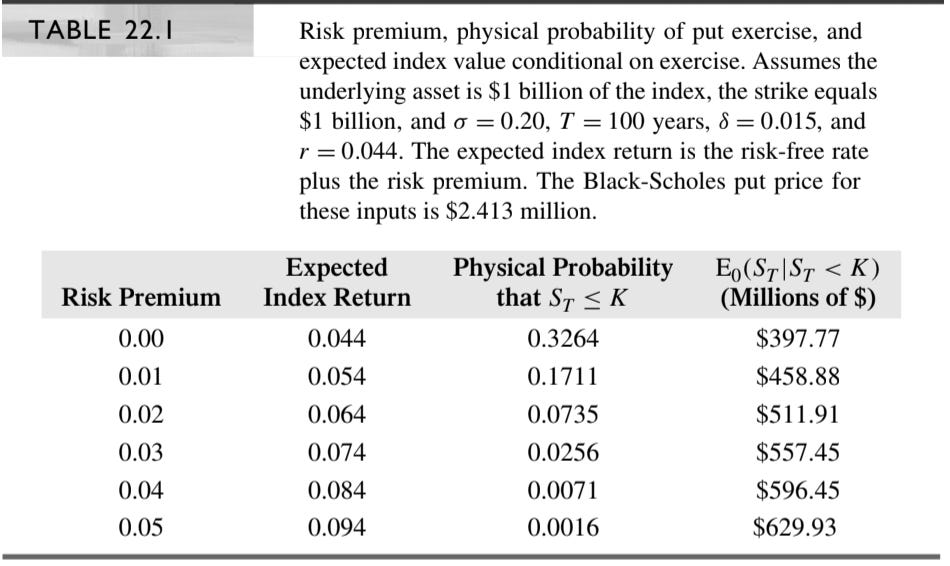
It cannot be stressed enough that Buffett wasn’t discussing the risk-neutral probabilities of Black–Scholes but rather real, actual probabilities. If we also use real probabilities, we arrive at figures consistent with Buffett’s approximation. Assuming an equity index risk premium of 4%, we indeed obtain a probability of less than 1% that the market ends below its starting level in 100 years. In addition, under a log-normal model, conditional on the market ending below its start, its value would be 59.6% of the current index—again close to Buffett’s 50% assumption.
Buffett’s pronouncements on the long-term behavior of equity indices suggest an equity risk premium of approximately 4% and a total discount rate for equities of 8.4%. Under risk-neutral probabilities—where the risk premium is zero—the probability of the index falling below its initial value after a century approaches 33%. This discrepancy stems from the compounded effect of a 4.4% versus an 8.4% rate over 100 years, rather than, as Buffett contends, a misapplication of volatility in deriving true probabilities.
The 33% figure represents a risk-neutral probability, valid only within the risk-neutral measure and not to be conflated with real-world probabilities. Indeed, it is only by delta‐hedging that banks which sold the puts can eliminate directional risk and earn low‐risk profits. In effect, the banks were lending money to Berkshire Hathaway at a low rate (reasonable, given Berkshire’s credit standing). This case illustrates the pitfalls of naively interpreting option-implied probabilities without considering the risk-neutral framework in which they are derived.
What Buffett Got Right
While Buffett’s decision to sell put options through Berkshire Hathaway was based on a misinterpretation of the probabilities implied by the Black–Scholes model, his brilliance showed in negotiating contracts that deferred potential loss recognition until his later years. His confidence in the resilience of major global stock markets proved profitable, but it’s important to note that selling puts isn’t universally applicable—its probability of success increases with option maturity.
Moreover, Buffett noted using put premiums to purchase stock, effectively transforming the position into leveraged exposure to the equity risk premium. Indeed, a call option (equivalent to buying a put plus buying the underlying) is itself a leveraged bet on the asset (the underlying is a zero-strike call). Because a put has negative exposure everywhere, selling the put and buying the stock creates even higher leverage on the underlying than a long call.
In any case, modest leverage on broad market exposure has historically enhanced long-term returns. Leverage amplifies the equity risk premium—which has outpaced risk-free rates—while compounding returns over time. It also aligns with the efficient market hypothesis: broad indices efficiently incorporate information and economic growth, and their diversification mitigates idiosyncratic risk, making leveraged index exposure potentially less risky than picking individual securities.
So it turns out that Buffett was right after all: buying major indices on leverage can be profitable. Yet framing matters. Challenging established models like Black–Scholes often attracts more attention than advocating simple strategies like modestly leveraged index investing. It’s also crucial to recognize that the institutions trading with Buffett weren’t misguided—they generated low-risk profits via dynamic delta hedging, while Buffett assumed the equity risk premium. That premium materialized in the U.S. market, but such outcomes aren’t guaranteed across all markets or time.
The Purpose of Equity Derivatives
Derivative are fundamentally nothing more than dynamically replicated payoffs whose prices are set in the risk-neutral world. Issuers construct caps, buffers, barriers, or other features by continuously trading the underlying and financing positions so that, in a frictionless model, the resulting payoff exactly matches the promised structure. The fair value of these products emerges from the cost of that dynamic hedging under the assumption that all assets earn the risk-free rate—i.e. in the risk-neutral measure—rather than their actual expected returns.
In reality, investors live in the “physical” or real-world world, where broad equity indices earn a positive risk premium above cash. When a structured note is fairly priced via risk-neutral replication, it nonetheless delivers real-world upside roughly in line with that equity premium—because the note’s payoff still remaps the same underlying returns, it merely shifts probabilities between scenarios. For example, a buffered note that protects the first 20% of losses will pay out nearly 100% of market gains above that buffer, so if the S&P 500 returns 8% annually over a decade, the investor captures most of that return, less a small financing cost embedded in the note’s price.
Thus, when structured notes and options trade at fair, arbitrage-free prices, they do nothing mystical to expected returns—they simply “sculpt” the distribution of outcomes. Investors effectively exchange a sliver of extreme upside for a controlled floor on losses (or the other way around), all at a cost precisely equal to the replication expense. In doing so, these instruments elegantly tailor downside risk to match risk preferences, while preserving the vast majority of long-run equity gains that arise from the real-world risk premium.
Disclaimer
The information provided on TheLogbook (the "Substack") is strictly for informational and educational purposes only and should not be considered as investment or financial advice. The author is not a licensed financial advisor or tax professional and is not offering any professional services through this Substack. Investing in financial markets involves substantial risk, including possible loss of principal. Past performance is not indicative of future results. The author makes no representations or warranties about the completeness, accuracy, reliability, suitability, or availability of the information provided.
This Substack may contain links to external websites not affiliated with the author, and the accuracy of information on these sites is not guaranteed. Nothing contained in this Substack constitutes a solicitation, recommendation, endorsement, or offer to buy or sell any securities or other financial instruments. Always seek the advice of a qualified financial advisor before making any investment decisions.