Factor Investing

Most factors probably wont work, but a few will work very well

Aug 22, 2024

Factor investing has been around for a while and there is an immense literature devoted to it. Yet, much confusion and misconception remain, even among practitioners. In this post, we introduce factor models in a self-contained way as well as present an overview of the current state of research. Sources for this post include Advanced Portfolio Management (APM) by Giuseppe Paleologo, two papers from AQR, and two articles from Chicago Booth Review.

A One-Factor Model

A factor in the context of stock return models is a measurable characteristic or variable that can explain or predict a stock's return (conversely, a factor would also explain or predict a stock’s risk). For example, the most common one-factor model for predicting returns would be to use the market factor. One would expect a cyclical stock in the financial sector like Synchrony Financial (SYF) to move more in sync (pun intended) with the market than Walmart (WMT) which is a large, stable, defensive stock. The figure below from APM show the regression of SYF and WMT daily returns against S&P 500 futures from January 2 2018 to December 31 2019.

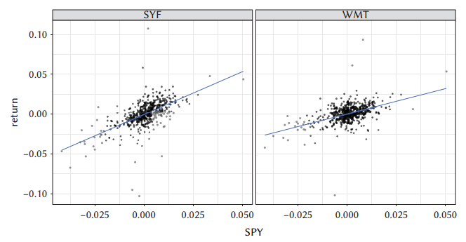
Decomposing stock returns into market and stock-specific components offers crucial insights. This analysis reveals what fraction of a stock's return is attributable to market movements, potentially uncovering counterintuitive performance trends. For instance, a stock seemingly outperforming in a bull market might actually be underperforming once its high market sensitivity is accounted for (note that SYN has higher slope but lower intercept to WMT). The complete formula for the relationship between stock and market returns is

\(r = \alpha + \beta \times m + \epsilon \)

where r is the stock return, α is the intercept, β is the stock's market sensitivity, m is the market return, and ε is the idiosyncratic return or "noise". The β × m term represents the systematic return, while α + ε comprises the stock-specific return. Alpha represents the expected stock return when market return is zero, though realized returns always include the noise term ε.

This model, known as a single-factor model, assumes that all commonalities among stocks come from their market sensitivity (beta). The idiosyncratic component (α + ε) is company-specific, potentially allowing for diversification of this "noise" across multiple stocks. Taking the expectation of this equation yields the expected stock return as a function of alpha, beta, and expected market return.

Different investment professionals focus on various aspects of this model. Fundamental investors aim to estimate α accurately, quantitative risk managers focus on β and identifying appropriate benchmarks, while macroeconomic investors attempt to forecast market returns. Portfolio managers must synthesize all this information for effective portfolio construction.

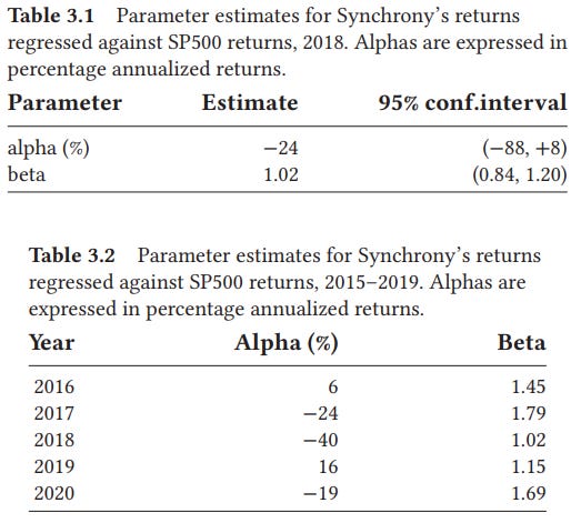
Alpha is challenging to estimate accurately, as historical data shows large confidence intervals and high variability over time. Unlike beta, which tends to be more stable, alpha estimates are often unreliable when derived from time series data alone. See estimates of beta and alpha for SYN below from APM:

The task of predicting forward-looking alpha values falls to fundamental analysts, who rely on deep research and various data sources. This process, known as alpha generation, is of course non-trivial (as people get paid a lot to do it well).

The flip side is that if you are someone with money to invest, then finding alpha is expensive for you. One of the most significant insights in modern portfolio management is that generating returns doesn't necessarily require alpha (stock-specific outperformance). Instead, investors can focus on identifying "factors" that represent independent sources of risk beyond the market itself. These factors, when properly identified and leveraged, can potentially lead to returns that compensate for the additional risk taken.

From One to Many

The evolution of factor models in finance is a fascinating journey that began with the Capital Asset Pricing Model (CAPM) in the mid-1960s. Initially proposed independently by Lintner, Mossin, and Sharpe, the CAPM introduced the concept of market beta as the primary factor explaining stock returns. This model was supported by empirical studies in the early 1970s (for which its creators later received Nobel Prizes).

The mid-1970s saw a natural extension of this thinking, driven by three young researchers. Stephen Ross, then at Yale, extended CAPM by proposing that multiple factors—not just market beta—could influence stock returns. This led to the development of what became known as the Arbitrage Pricing Theory (APT). Concurrently, Barr Rosenberg and Vinay Marathe at Berkeley suggested that stock characteristics, such as financial ratios, could serve as factor loadings, introducing the idea that company-specific attributes might systematically affect returns.

The third key contribution came from Rolf Banz at Northwestern, who provided empirical evidence challenging CAPM. His research showed that small-cap stocks tended to outperform large-cap stocks, suggesting that market capitalization was an important factor beyond market beta in explaining stock returns.

These developments laid the groundwork for multi-factor models in finance. Their impact was profound, both in academia and in the investment industry. Notably, Rosenberg went on to found several successful companies—including Barra (now part of MSCI)—which commercialized factor models. The advent of these multi-factor frameworks also coincided with technological advancements that made their practical implementation possible. In the early 1980s, handling the massive amounts of data required for comprehensive stock analysis was challenging. Since then, the field has exploded with the discovery of numerous factors explaining equity returns, and the same approach has been successfully applied to other asset classes.

Now, instead of just having one factor, an equation a risk-manager uses to explain returns may look like the following:

\(r = \alpha + \beta_1 \times f_1 + \beta_2 \times f_2 + \cdots + \beta_m \times f_m + \epsilon\)

where each beta is a factor loading to one of the m factor returns. While many factors in multi-factor models are interpretable and grounded in economic or financial theory, it must be noted that they are often not directly tradable assets.

This non-tradability arises for several reasons. First, some factors—like size or value—are abstract concepts rather than specific securities. They represent characteristics of stocks but aren’t standalone investment vehicles. Second, factors may be composite measures derived from multiple data points, making them challenging to replicate exactly in a portfolio. Third, even when factors are based on observable metrics (such as the book-to-market ratio), creating a pure exposure to that factor while eliminating all other exposures is practically difficult. Fourth, transaction costs and market frictions can make it prohibitively expensive to maintain a portfolio that perfectly tracks a factor, especially for factors requiring frequent rebalancing. Lastly, some factors may rely on proprietary methodologies or alternative data sources, further complicating direct replication.

Types of Factors

Many factors were initially introduced to address anomalies unexplained by the Capital Asset Pricing Model (CAPM). There are two primary explanations for non-zero factor returns. The first is risk-based: these returns compensate portfolio managers for bearing specific risks that are independent of market risk. This view aligns with market efficiency, where all risks are appropriately priced. The second is behavioral: factor returns arise from investors’ bounded rationality, cognitive biases, and limited information processing capabilities. Both perspectives are relevant—the risk-based view is crucial for risk management, while the behavioral lens aids in factor interpretation.

Factors have proliferated rapidly in both academic literature and practical applications. Commercial risk-model providers often include dozens of factors—typically between 50 and 100—to ensure comprehensive coverage of potential risk drivers. When you examine the correlation matrix of these factors, distinct clusters emerge. Common groupings include industry-specific clusters (such as financials, healthcare, and consumer retail) and broader market factors (like overall market sensitivity and volatility). These clusters and their interrelationships often have intuitive economic explanations.

I now quote directly from APM for the following:

Group #1 shows positive correlations between two clusters of production inputs: “metals and mining,” “chemicals,” “construction materials” on one side, and “paper and forest products” through “construction engineering” on the other.
Group #2 shows that these same industrial outputs are positively correlated with market factors—that is, these industries are cyclical.
Group #3 shows that financial industries are also cyclical.
Group #4 reveals a positive correlation between cyclical industries connected via supply-chain relationships (products and their retail channels): “consumer durables,” “autos,” and “auto parts” on one side, and “multiline retail,” “distributors,” and “luxury goods” on the other.
Groups #5 and #6 show that utilities and consumer staples industries are negatively correlated with market-factor returns, consistent with their status as defensives.

Not all factors consistently generate positive returns. In fact, returns associated with different factors can vary significantly over time, and some factors may even exhibit negative returns in certain periods. When a factor does consistently produce positive returns over the long term, this phenomenon is referred to as a factor premium or risk premium. A factor premium represents the additional return investors can expect to earn by being exposed to that particular risk. For example, the “value premium” refers to the historical tendency of value stocks (those with low price-to-book ratios) to outperform growth stocks over long periods.

However, factors can be valuable for risk management purposes regardless of whether they offer a premium. Their utility in risk management stems from their ability to explain and decompose the sources of risk in a portfolio, rather than solely their potential to generate excess returns. Below we describe the factors deemed most material, experimentally robust, investable, and interpretable:

Country (Market) Factor
The country factor—often called the market factor—is the most fundamental element in factor models. It acts as a binary baseline factor (either 1 or 0); in single-country models, its returns closely approximate the average returns of all stocks traded in that market. Multi-country or regional models (covering areas like Europe, Asia Pacific, or North America) typically feature one country factor per region (or per country where exposures differ materially). This factor generally exhibits positive expected returns, as it represents the equal-weighted average of asset returns on any given day.
Industry Factors
Industry factors extend the country-factor concept within a given universe. In a global model, countries partition the global universe; in a country-specific model, industries partition that country’s universe. There is typically one factor per industry, with stocks having unit exposure to their own industry and zero exposure to others. This pure industry exposure differs from a simple capitalization-weighted industry portfolio (like a sector ETF), as it strips out style-factor effects and isolates industry-specific dynamics.
Beta (Market Sensitivity) Factor
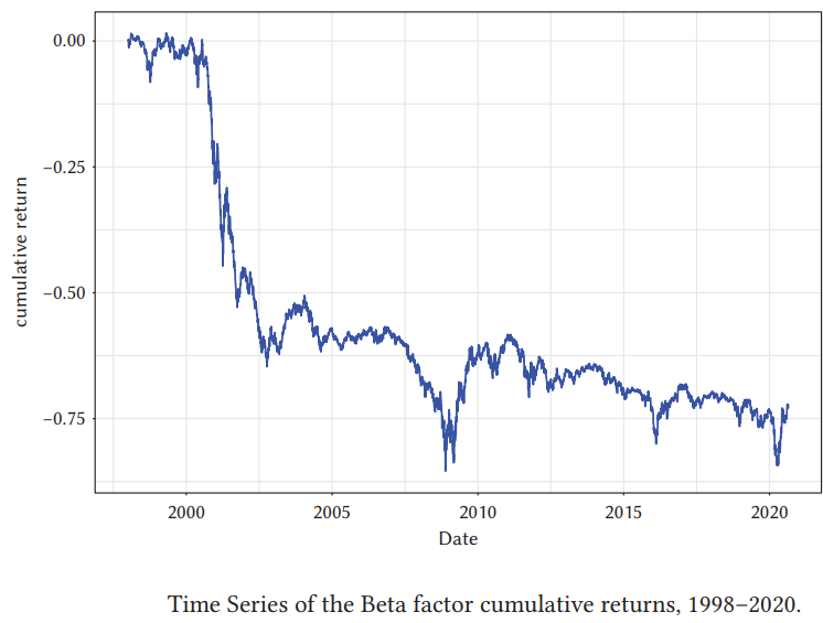
This factor should not be confused with a stock’s beta exposure to the market. Here, the factor return is defined as the P&L of a dollar-neutral portfolio that is long high-beta assets and short low-beta assets (using, for instance, the S&P 500 in the US). By CAPM, one would expect this portfolio to have positive returns, since high-beta assets exhibit greater sensitivity to a market with positive expected returns. Empirically, however, betting against beta is often profitable. One explanation is that many investors (e.g., pension funds) face constraints against shorting or using leverage. To chase returns, they overweight high-beta stocks (or private-equity-like assets), creating excess demand and driving prices above intrinsic value. Over the long run, this overpricing leads to negative returns for the high-beta segment. See graph from APM.

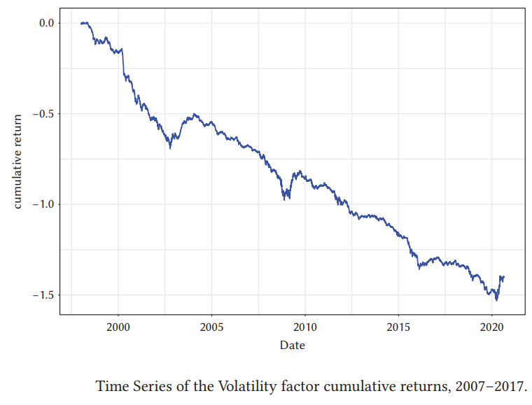
The volatility factor is closely related to the beta factor, and its returns are defined as those of a dollar-neutral portfolio that is long high-volatility stocks and short low-volatility stocks. There is a direct relationship to the beta factor, since beta itself depends on a stock’s volatility. From regression, we know that

\(\beta = \rho \times \frac{\sigma_i}{\sigma_m}\)

Where ρ is the correlation of the stock to the market, σᵢ is the stock’s volatility, and σₘ is the market’s volatility. Since σₘ is common to all stocks, if every stock shared the same ρ, beta and volatility factors would be perfectly proportional and thus indistinguishable. In practice, correlations vary across stocks, and it remains an open question whether those differences render beta and volatility truly distinct factors. Regardless, the empirical evidence is clear: a dollar-neutral strategy that is long low-volatility stocks and short high-volatility stocks—while remaining neutral to other major factors—tends to generate positive returns. In other words, systematically “shorting” the volatility factor has historically been profitable. See graph from APM.

Most attempts to explain the low-volatility anomaly fall into two categories:

Portfolio manager incentives. Their compensation structure (2% of AUM, 20% of returns above benchmark) effectively turns their careers into one large call option: there’s a floor—poor performance costs them their jobs—but no ceiling on upside (“silly” pay for strong gains). This asymmetric payoff inflates demand for volatile stocks.
Factor overlap. The volatility factor can be decomposed into other well-known factors—chiefly profitability (e.g., earnings-to-price) and value (book-to-price). In other words, low-volatility stocks often coincide with high-profitability and value stocks, both of which have historically delivered positive returns.

While many retail investors chase high-volatility, high-beta stocks hoping for outsized gains, a strategy of buying more stable businesses and judiciously applying leverage can yield superior risk-adjusted returns over time. This approach—famously favored by Warren Buffett—leverages the tendency of well-managed, durable companies to outperform on a risk-adjusted basis.

The Short Interest factor can be measured in a few different ways, short ratio, short-to-float, days-to-cover, utilization rate, borrow cost, etc… It is debated whether there is a persistent negative premium associated with short interest.

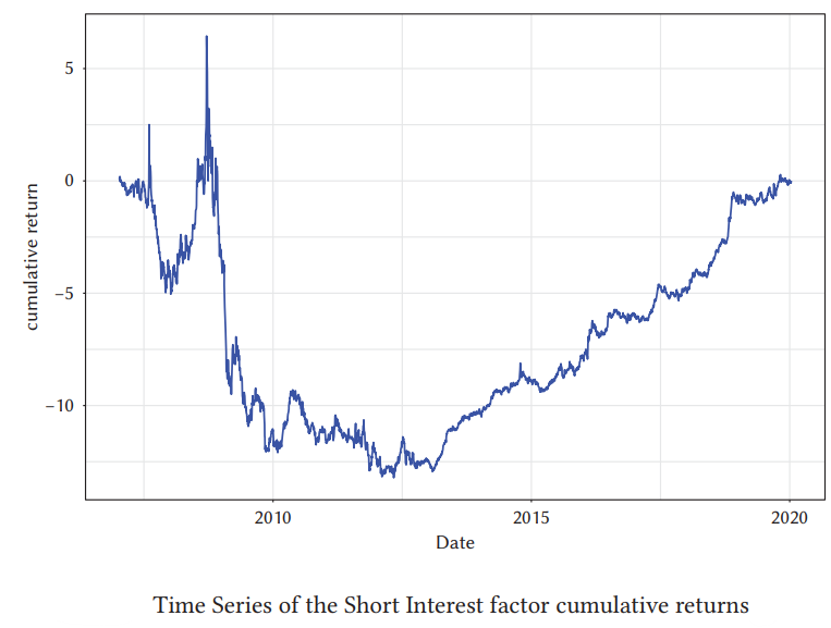
While simple models that use only the short-interest factor—or combine it with the market factor—don’t typically exhibit a persistent negative risk premium, practitioners have found that including short interest in more sophisticated multi-factor frameworks can add significant predictive power. Fundamentally, heavy short interest signals that sophisticated, well-capitalized investors believe a stock is overpriced and have the resources to drive the price lower. In effect, short interest captures the informed views of market participants who are able to act on their convictions, making it a valuable addition to complex risk models.

The Active Manger Holdings factor is the positive counterpart to the short interest factor. There is variation across active investors, but there is commonality as well, and it is captured by this factor. In some sense, like the short interest factor, AMH can be interpreted as a measure of “crowding”. Again, it is debated if a premium exists.

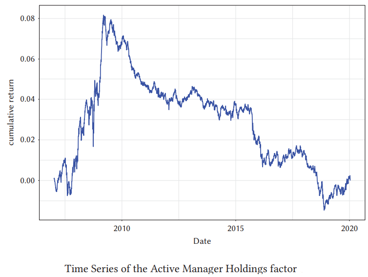
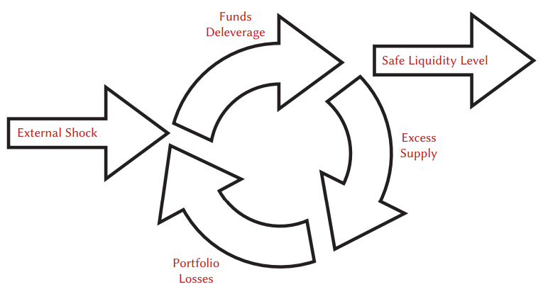
In the absence of external shocks, crowding can be beneficial to returns: as different portfolio managers bid up the same stocks, consensus positions earn a premium. However, if an adverse event triggers sufficiently large losses, holders of these crowded positions may deleverage, causing further price declines and forcing yet more deleveraging—a vicious cycle. The same dynamic affects crowded shorts: in a distress event, short sellers scramble to cover their positions, driving the stock price higher, much like a crowd rushing for the exit in a theater. Thus, regardless of whether factor premiums exist, both short interest and the adaptive markets hypothesis are crucial for understanding the risks inherent in crowded trades.

The Momentum Factor of a stock is given by its past performance over a given interval compared to its peers. Momentum is a robust anomaly and has been observed in markets over different asset classes (equities, commodities, bonds) and over long time intervals (two centuries). The reason for its continued outperformance therefore cannot be ascribed to characteristics of stocks alone.

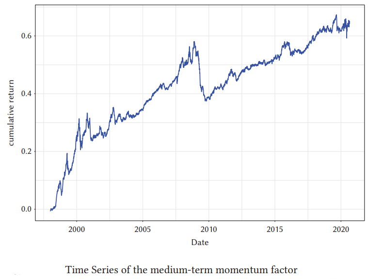
The most frequent explanations given for momentum are investor overreaction and investor underreaction (yes, you read that right). Perhaps investors underreact to news because they are overconfident or inattentive, creating a lag between fundamental changes and prices reflecting them. But then, of course, investors may overreact to returns, extrapolating them into the future, generating additional demand and further optimism that pushes the price up. A cursory read of the research on momentum will convince the reader that no one truly understands its origins—though practitioners are happy that it exists.

All we have are hard-to-falsify theories based on observational data. Indeed, in addition to behavioral explanations of momentum, the last decade has seen the emergence of risk-based theories: that momentum returns compensate for tail risk. This view is drawn post hoc from the observation that momentum, while profitable, experiences strong, sharp reversals.

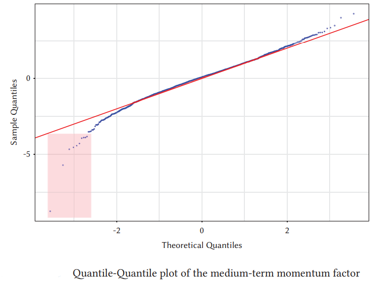
In addition, momentum risk in factor investing is more complex than it might initially appear, particularly because momentum portfolios are typically constructed as dollar-neutral long-short strategies. This means risk arises from both the long and short sides of the portfolio. On the long side, the traditional concern is that stocks exhibiting strong upward momentum may be in a bubble—and thus vulnerable to sudden reversals and crashes, leading to significant losses. Equally important, and often overlooked, is the risk on the short side: stocks that have underperformed (and are therefore shorted in a momentum strategy) can rebound sharply—especially during market recoveries following steep downturns—resulting in large losses on the short positions.

The characteristic most frequently used to measure the value factor is the book-to-price (B/P) ratio. However, this metric is increasingly outdated in an economy where much of a company’s value resides in intangible assets. As a result, “value” is often defined using alternative ratios—sales-to-price, free-cash-flow-to-price, earnings-to-price, EBITDA-to-enterprise-value, dividend yield, net income, and so on. Indeed, fundamental investors have employed a wide array of intrinsic-value metrics since the dawn of value investing, raising the risk of overfitting. Depending on how “value” is defined, a dollar-neutral long-short portfolio can exhibit either a positive or negative premium.

By definition, a stock that is low on value is either overpriced or has priced in a much higher rate of growth. As such, the opposite of the value factor can be defined as the growth factor. The formula linking value to growth is

\(\frac{\text{cash flow}}{\text{price}} = \frac{\text{rate of return - growth rate}}{\text{payout ratio}}\)

There are many possible explanations for why and how value and growth work. Like momentum, the empirical evidence on the subject is not conclusive. In one sense, value and growth together can be interpreted as duration exposure in the portfolio. Growth stocks derive most of their value from cash flows far into the future—much like long-term bonds. Value stocks, conversely, resemble companies under distress, with a much shorter time horizon; their valuation is realized sooner. One would therefore expect the term spread (the difference between long-term and short-term bond yields) to be correlated with value-factor returns—and, indeed, this has been observed.

In another sense, assuming markets are efficient, value stocks aren’t “cheap” because they offer a bargain but rather because they are riskier. From this perspective, value stocks are intrinsically riskier than growth stocks: they’re more likely to experience earnings or dividend shocks (per the options market) or face financial distress. Both phenomena have been documented: value-stock portfolios tend to consist of firms with high fixed costs, unproductive capital, and complacent management. This generates greater downside risk during recessions without a commensurate upside in expansions.

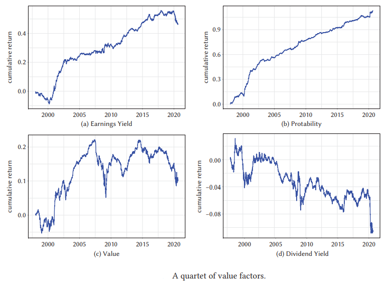
The carry factor is a cousin of the value factor: it captures returns from borrowing in a low-yielding asset and lending in a high-yielding one (the classic example being funding in a low-rate currency and investing in a high-rate currency). Returns are positive if prices remain unchanged.

In fixed income and commodities, a carry strategy sells futures in contango and buys them in backwardation; in equities, carry is simply the dividend yield, which exhibits distinct cumulative returns from other value metrics. At its core, carry trades exploit interest-rate differentials—borrowing in low-rate currencies to invest in high-rate ones—capitalizing on the fact that Uncovered Interest Rate Parity often fails in the short to medium term. The higher rates in target currencies act as a risk premium for political and credit risk. Carry factors tend to perform well when global risk appetite is strong and central banks maintain persistent rate differentials. However, they can suffer sharp reversals during sudden shifts in market sentiment or stress.

An Excess of Factors

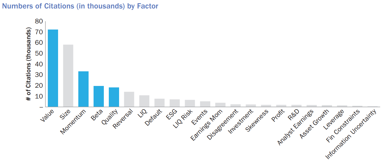
By now it should be clear that the discovery and publication of factors which explain the cross-section of expected returns can be a profitable endeavor to fund managers and academic alike (maybe not always to investors). Indeed, the finance industry has a habit of going into cycles where good ideas become products.

Researchers have identified over 400 factors in academic literature; suggestions to explaining returns discrepancies range from the facial attractiveness of fund managers to the weather in New York City. While factors can help create truly balanced portfolios, there’s skepticism about whether all these factors are genuinely useful or if many are redundant. The concerns are twofold: (1) some factors may be the result of data-mining (the industry standard t-statistic threshold is 2), and (2) some factors may describe the same underlying risk exposure.

The first point can be addressed by raising the required level of statistical significance, as noted in “The Cross-Section of Expected Returns.” However, financial data is often only available monthly or quarterly, making high statistical significance difficult to achieve; recall that the standard error of the sample is proportional to the reciprocal of the square root of the number of observations.

To illustrate the second point: researchers have found that the excess premium for momentum is no longer statistically significant over some periods after accounting for left-tail risk. In effect, these two risk factors describe the same phenomenon during the observed timeframe. This doesn’t necessarily change how portfolio managers operate—indeed, many so-called “new” factors may simply be subsets of already-discovered ones. Redundancy can be hard to spot because new factors are often evaluated only against a limited benchmark model. For example, a liquidity factor might really be capturing the same effect as the well-established size factor (small-cap stocks are also typically less liquid than large-cap ones).

It may be tempting to use the entire set of existing factors as a benchmark when evaluating new ones. But with limited data, the curse of dimensionality undermines statistical significance. One study of 99 of the most cited factors over the past decade found that only 13 held significant explanatory power—underscoring the need for skepticism when assessing the hundreds of factors in the academic literature.

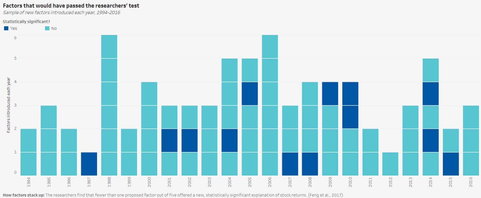
The proliferation of factors may be partly driven by academic publication pressures, which demand specific significance thresholds (p-values) for acceptance. This can incentivize data mining or “p-hacking” to achieve publishable results—a manifestation of Goodhart’s law: “when a measure becomes a target, it ceases to be a good measure.” In practice, researchers may inadvertently present spurious patterns as statistically significant without a solid causal hypothesis.

That said, our critique of redundant factors should not be mistaken for an endorsement of an overly parsimonious model that explains stock returns with just a handful of factors. The pursuit of simplicity in finance often reflects “physics envy”—the wish to emulate the elegance and predictive power of models from the physical sciences. Yet financial markets, driven by human behavior, resist such neat reduction. By acknowledging our ignorance, we embrace a more humble, realistic—and ultimately more scientific—approach to finance. This mindset encourages us to leverage what we know while remaining cautious about what we don’t, fostering more stable and resilient financial systems and practices.

Premium and Diversification

We now summarize results from AQR research on the 4 most well-established factors. We ignore the size factor here because although there is much publication about it, its current existence is under intense debate.

These are factors that we have previously discussed. Value is the tendency for cheap assets to outperform expensive ones, momentum is the tendency for recent performance to continue into the near future, carry is the tendency for higher-yielding assets to provide returns above those of lower-yielding assets, and defensive is the tendency for low beta stocks to outperform on a risk-adjusted basis. Each factor lends itself both to risk-based and behavioral explanations:

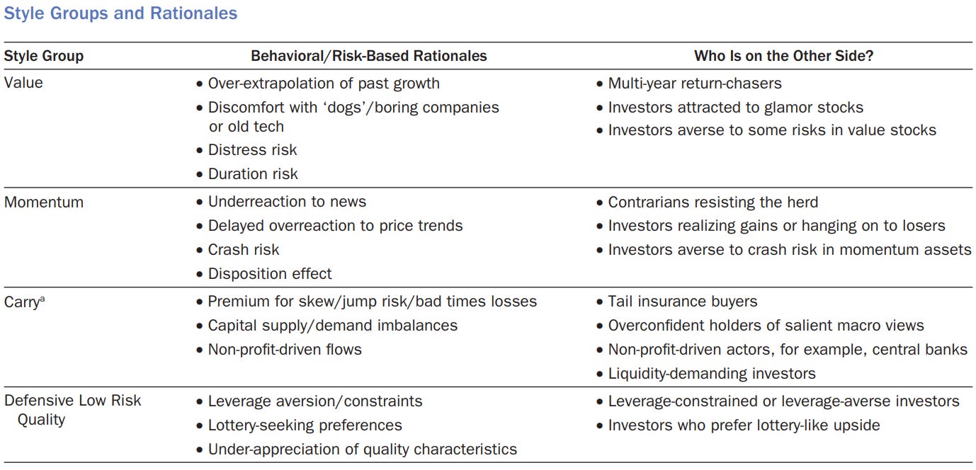
In addition to the potential for earning risk premiums, factors can provide exposure to different sources of risk and return that may have low correlations with each other and with traditional asset classes. This multi-dimensional diversification can potentially improve the risk-adjusted returns of a portfolio, even if some factors do not consistently deliver positive premiums.

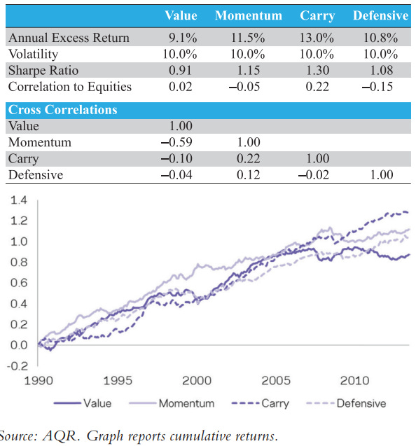
By combining factors that respond differently to various market conditions and economic cycles, investors can create more robust portfolios that are potentially better equipped to weather diverse market environments. For instance, value and momentum factors often exhibit negative correlation, providing a natural hedge within a portfolio. Factor diversification can help mitigate the impact of factor cyclicality, as different factors may outperform at different times.

While factors have gained popularity in investment strategies and academic research, it's crucial to understand that at the end of the day, if you believe in the risk-based explanations, that they can deliver returns only by exposing you to risk (albeit it be uncorrelated risk to the market). Historical data may show long-term premiums for certain factors, but these premiums can disappear or reverse for extended periods (for example, with size), sometimes lasting years or even decades.

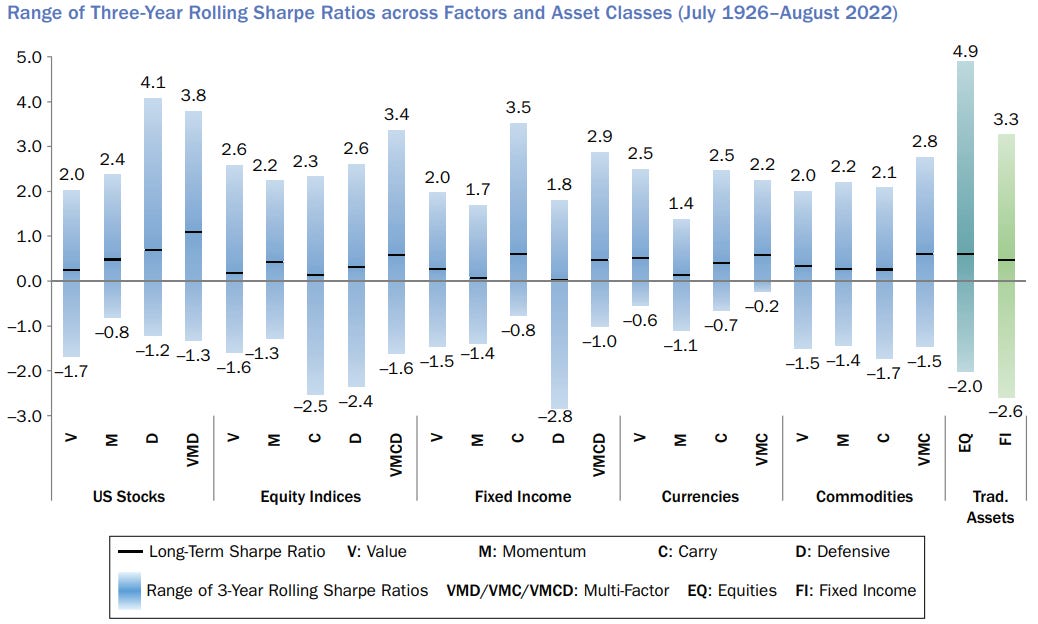
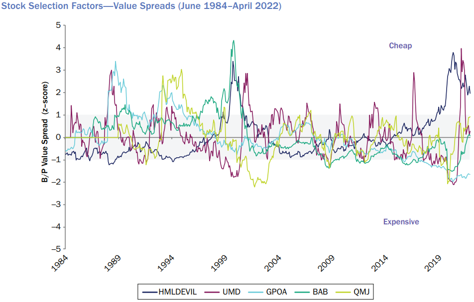
Factors can experience significant drawdowns, volatility, and periods of underperformance relative to the broader market. Moreover, as factors become widely known and adopted, their effectiveness may diminish due to crowding or changes in market dynamics. Below, we plots the time series of valuation spreads of value (HMLDEVIL), momentum (UMD), profitability (GPOA), defensive (BAB), and quality (QMJ) factors. The value spreads indicate whether a factor looks “cheap” or “expensive” relative to its history:

Additionally, transaction costs, taxes, and implementation challenges can erode the theoretical benefits of factor strategies in practice. For example, as a value stock realizes its value and appreciates in price, it is no longer a value stock by definition. Finally, the reader can probably discern that factors are fundamentally ideas that can be captured by a range of financial metrics. A factor such as “value” can especially be difficult to defined in an economy where much of the cashflow of a company is derived from its intangible assets.

Portfolio management is fundamentally a craft, a blend of art and science that defies simple codification in any single book or rigid set of rules. It's a dynamic discipline that continually evolves in response to changing market conditions, emerging technologies, and shifting economic paradigms. The nuances of effective portfolio management are often learned through years of hands-on experience, adapting to market cycles, and navigating complex, sometimes unprecedented scenarios. What worked in one market environment may prove ineffective in another, requiring managers to constantly refine their strategies and approaches. It is a living, breathing practice that requires lifelong learning and adaptation, far beyond what any static text can fully capture.

Discussion about this post

Ready for more?