
The Risks of a Growth Efficient Portfolio
Also, What Exactly is Volatility Drag Doing?

Kelly strategies that employ leverage have the ability to consistently outperform over extended time horizons. However, in this post we explore their significant trade-off in the form of risk. Numerical examples come from this PIMCO Paper mentioned in the previous post.
Introduction
Leveraged strategies — especially when expressed through ETFs — are often pitched as shortcuts to “amplify” market returns. The math seems simple: if the S&P 500 goes up 10%, a 2x ETF should give you 20%, right? But beneath the surface, leveraged portfolios hide a subtle yet powerful enemy: volatility drag. Investors are quick to blame “fees” or “decay,” but few understand the precise mechanical reasons why leveraged products so often disappoint in practice — even when the market moves in your favor on average.
This post aims to peel back the layers and dissect exactly how volatility erodes geometric returns, how rebalancing rules create negative gamma effects (forcing you to buy high and sell low), and how even theoretically “optimal” growth strategies like Kelly betting can become fragile when exposed to real-world paths and estimation errors. We’ll explore why most of the outperformance from leveraged approaches actually comes from rare, uninterrupted bull markets — and why in most realistic scenarios, these strategies lead to worse median outcomes than investors expect.
Finally, we’ll connect this to practical solutions: how structured products and customized payoff profiles (especially on-chain) can help shape risk more intelligently, allowing investors to avoid the blind spots of naive leverage while still accessing upside potential. If you’ve ever wondered why your leveraged ETF doesn’t match the chart, what’s really happening behind “volatility decay,” or how to build a strategy that aligns with your real-life goals instead of just chasing textbook optimality, this deep dive is for you.
Growth Efficient Frontier
Due to the effects of volatility drag, the geometric growth rate of a portfolio that allocates a proportion x (where x can be greater than 1) to the risky asset is given by
This function is a concave-down parabola, implying that there is a point of optimal leverage that maximizes the geometric growth rate. It also means that excessive leverage beyond this point actually reduces the growth rate.
Assuming that r = 1.8%, μ = 3.2%, and σ = 15% the “growth efficient frontier” of various values of x is shown below (x ranging from less than 0 to greater than 1):
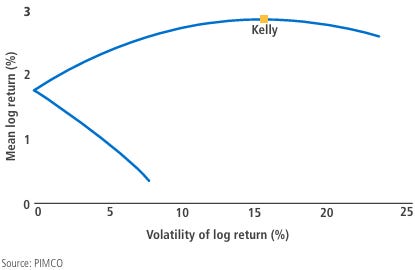
We note that on a quadratic curve, the slope of the tangent line approaches zero as we approach the vertex. In other words, the frontier becomes almost flat near the maximum, implying that slightly reducing expected log returns can significantly lower risk, as measured by volatility. Most investors are more risk-averse than implied by log utility, and thus would naturally allocate at a leverage significantly below the theoretical growth-optimal point.
Risks of the Optimal Growth Portfolio
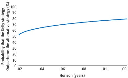
We consider a few important aspects of the optimal growth (Kelly) portfolio. First, although the Kelly strategy dominates other strategies in the long run, it can take a very long time for this dominance to materialize.
For example, in the case of r = 1%, μ = 4%, and σ = 15% it would take 227 years to have a 90% confidence that the Kelly strategy (x=1.3) will outperform the alternative low-risk strategy with x=0.2:
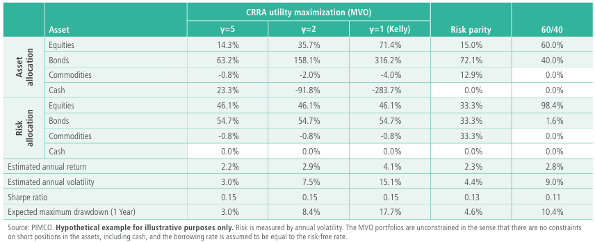
Now consider additional risks associated with the Kelly portfolio, using results drawn from the PIMCO paper mentioned previously (under the same assumptions).

First, we see just how aggressive Kelly allocations can be: in this example, 71% equities and 316% bonds, implying borrowing roughly 3x the portfolio’s value.
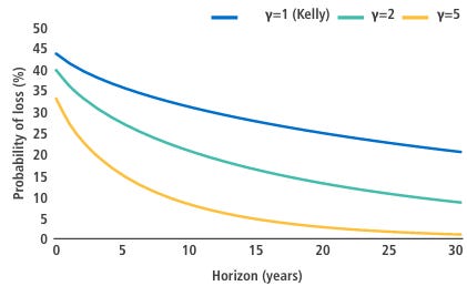
The probability of loss over a 30-year horizon is nontrivial.
The expected maximum drawdown (largest peak-to-trough decline) can approach 25% in a single year, highlighting the short-term risk.
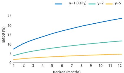
In addition to these quantitative drawbacks, the Kelly portfolio is also highly sensitive to estimation errors in return distributions, since the weight in risky assets is directly proportional to the excess return and inversely proportional to the investor’s risk aversion parameter γ. In practice, Kelly portfolios tend to concentrate heavily in a few investments and often endure frequent and large short-term losses in exchange for superior long-term growth.
Negative Gamma of Leverage
The realized performance of a leveraged portfolio is reduced by volatility drag — the compounding penalty imposed by fluctuations in portfolio value. Rather than describing this drag purely to abstract variance terms, we now turn to understand the mechanisms that cause this underperformance.
Specifically, we explore how the rebalancing behavior required to maintain constant leverage introduces structural costs — including the adverse trading patterns we can characterize using concepts like negative gamma.
Indeed, it is intuitive that the geometric growth rate decreases with risk, and perhaps also intuitive that it should decrease proportionally to the square of how much the underlying moves around (i.e., volatility), as suggested by the simple quadratic term in the geometric return formula.
But what about negatively leveraged positions? At first glance, we might expect that a -1x short position should experience the same level of “volatility drag” as a +1x long position. However, careful consideration of how short positions are continuously hedged shows this is not the case.
Assume that you have a fund V that has unit net asset value (NAV) that wants to track an underlying S with leverage X. Your initial Δ (defined as dV/dS) is X. But then from time 0 to time T, S moves by some amount dS. We now aim to determine the Gamma (defined as dΔ/dS) of the portfolio. Take a second to think about this.
Assuming unit NAV, you start with X units of S for your exposure. After the asset moves, your NAV is now 1+XdS in dollars and you have X(1+dS) units of the underlying, i.e. your current Δ is X(1+dS). Your current leverage is therefore
In order to maintain a leverage of X you must target X(1+XdS) units of the underlying, i.e. this is your target delta. The trade you need to do to X(X-1)dS units of the underlying, exactly equal to the change in your Delta. Therefore, your Gamma, defined as the change in delta over change in underlying, is
The two elegant insights we can derive from this expression are that Gamma is proportional to the square of the leverage factor and that short positions have Gamma equivalent to that of long positions with one more unit of leverage. The graph of Gamma against leverage factor is an upwards sloping parabola with roots at 0 and 1.
To help internalize this, consider the example of -1x and +2x funds tracking an underlying S. Imagine S moves from 100 to 50, and then back to 100. Without rebalancing, both funds would be wiped out. If you had $200 total, splitting $100 into each fund, and rebalanced at 50, you'd end up with $150 (2x fund wiped out, -1x fund goes to $150; rebalance to $75 each; then -1x fund wiped out, 2x fund doubles to $150). By contrast, $200 invested directly in S would still be worth $200.
Thus, holding the underlying is not equivalent to holding a combination of 2x and -1x positions, even with periodic rebalancing. When you rebalance exposures outside the range [0, 1], you are forced to buy high and sell low to maintain target leverage.
Harvesting Leveraged ETF Gamma
One might observe a potential trade here: if borrowing costs are not too high, one could try to harvest negative gamma decay by shorting both positively and negatively leveraged ETFs (such as the 2x and -1x example). In principle, the shorting costs of leveraged funds should approximately reflect the implied volatility and expected "path-dependent decay" (volatility drag) of these products. If shorting costs are too low relative to this expected drag, there exists an arbitrage-like opportunity: you could short both the positively and negatively leveraged ETFs, effectively "harvesting" the volatility drag as excess return beyond what you pay to borrow. Conversely, if shorting costs are too high compared to expected drag, you could theoretically buy both, accepting the drag as long as it is less than the implied borrowing costs.
Of course, these trades are not without risk. A short position in a leveraged ETF can at most gain 100% if the ETF goes to zero, but a long position can, in principle, appreciate without bound, exposing you to unlimited downside if paired incorrectly. Moreover, large directional moves can force liquidations before this "drag capture" mechanism plays out. Nonetheless, in equilibrium, the market tends to price shorting fees so that they broadly align with the expected path-wise volatility decay, preventing easy arbitrage.
Log Returns & Volatility Drag
Building intuition for just how destructive variance (and higher moments) is to compound annual growth rate (CAGR) can be difficult. However, properly understanding log returns makes this clearer.
The relationship between your annual simple return and your log return is this: the log return represents the constant instantaneous rate you would need to achieve your annual return through continuous compounding.
Suppose you had a great year with a 100% simple return. If this return were achieved by compounding monthly, the required monthly growth rate would be around 6%.
When you naively annualize by multiplying 6% × 12, you get roughly 72%, which is much lower than the actual 100%. Alternatively, if you compounded daily to reach that same 100% return, you would need a daily growth rate of only about 0.3%.
When you multiply 0.3% × 252 trading days, you get just over 69%, which is close to ln(2). The key observation is that the more frequently you compound, the lower the growth rate you need to achieve the same simple return. This highlights how continuous compounding leads to larger terminal wealth given the same instantaneous growth rate.
For small returns, the difference is negligible. But as returns deviate further, especially on the downside, this difference becomes significant.
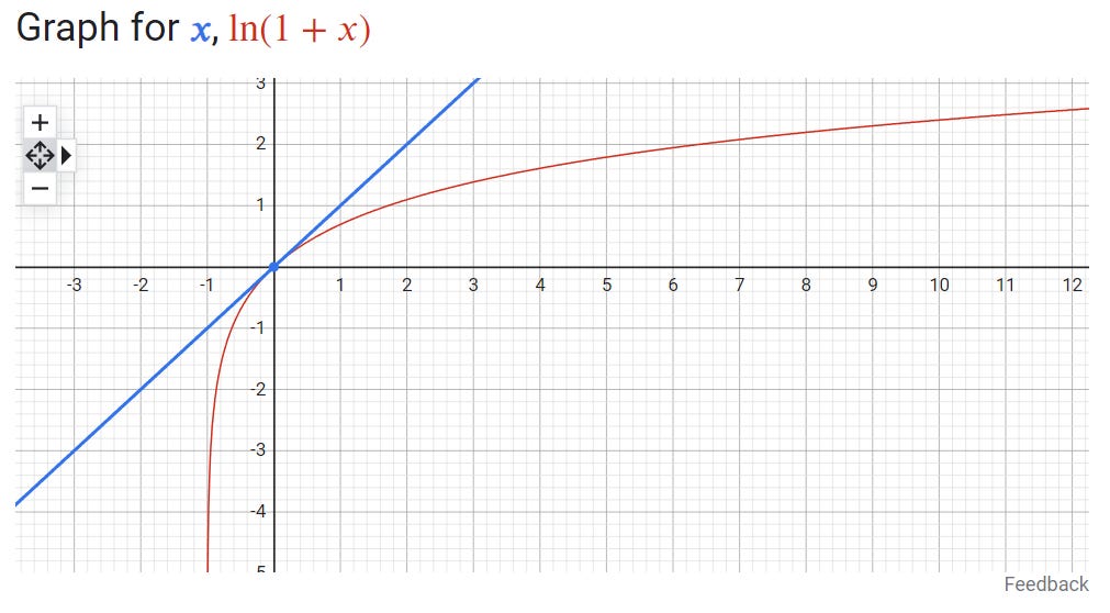
We know that variance increases the difference between arithmetic and geometric returns (CAGR = Simple Mean - Half of Variance), but the graph also illustrates that this impact is especially severe on the downside. Intuitively, if a price drops 50%, it needs a 100% gain just to break even. In log terms, a simple return of –50% corresponds to approximately –69% log return, while a +50% simple return corresponds to about +41% log return.
This highlights the non-linear relationship between compounded and simple returns: the natural log function quantifies just how asymmetric it is. Downside risks hurt disproportionately more than upside gains help — and beyond –100%, recovery is mathematically impossible, regardless of how large subsequent gains are.
Recall that a fundamental result in continuous-time finance is that any self-financing trading strategy can be seen as implicitly defining a contingent claim: by specifying your dynamic rebalancing rule, you determine a unique terminal payoff, regardless of whether you explicitly set a final payout function. In other words, every sequence of trades and re-hedges can be understood as "manufacturing" a payoff profile.
In the context of a growth-optimal (leveraged) portfolio, the so-called volatility drag we often view as harmful actually acts as a hidden form of downside protection and exposure on upside convexity. By rebalancing continuously to maintain constant leverage, the portfolio systematically reduces exposure after losses, decreasing the probability of total ruin (bankruptcy). On the upside, without rebalancing, your exposure naturally drifts back to 1 as the underlying rises, meaning you stop capturing additional upside beyond a certain point.
This trade-off is illuminated by considering the log return function ln(1+x) versus the linear return x. The log curve is concave and flattens quickly near zero, meaning that small daily (or frequent) rebalancing adjustments happen in a region where the gap between x and ln(1+x) is minimal. This local behavior allows frequent rebalancing to approximate smooth log compounding and avoid large deviation penalties. However, when rebalancing is too infrequent, the portfolio drifts into regions with large deviations between x and ln(1+x), magnifying the non-linear impacts of large moves and increasing downside ruin risk without the commensurate upside benefits.
Thus, by continuously rebalancing and accepting "drag," the portfolio gives up some median growth to improve tail outcomes: it better survives severe crashes and gain exponentially during bull runs. In effect, volatility drag becomes an implicit premium paid to manage convexity — akin to dynamically buying downside protection and exposing ourselves to runaway upside leverage.
In this sense, your self-financing rebalancing strategy creates a contingent claim profile that is effectively long downside convexity (to avoid bankruptcy) and long extreme upside convexity (to avoid unbounded exposure). Although we often emphasize that constant rebalancing forces you to buy high and sell low (classic negative gamma behavior), there are specific path cases where this seemingly adverse trading actually benefits you. Specifically, these are paths where you sell low — and it keeps going lower — or buy high — and it keeps going higher.
Do We Even Want Growth Efficiency?
On the surface, leveraged ETFs and Kelly-type strategies seem like the natural choice for aggressive investors seeking maximum growth. After all, they aim to maximize long-term geometric (log) returns and theoretically "dominate" lower-risk strategies given infinite time and no constraints. However, as we have seen in our analysis above, a large part of the realized outperformance in these strategies actually comes from extreme right-tail scenarios — those rare, uninterrupted bull runs where continually adding exposure compounds massive gains. While this sounds attractive, it also implies that most of the strategy’s edge is concentrated in a few improbable paths, rather than distributed broadly across typical outcomes.
For investors who care more about median outcomes — for example, those focused on ensuring robust retirement wealth or hitting a specific multi-year goal — these tail-heavy strategies can be deeply suboptimal. Leveraged ETFs also introduce constant negative gamma drag due to daily rebalancing, often locking in small losses and exposing investors to sharp drawdowns that can be psychologically or financially devastating. This is where structured products can offer an elegant alternative.
Rather than relying purely on leveraged linear exposure, structured notes and equity-linked certificates allow investors to explicitly shape their payoff distribution. For example, a leveraged equity-linked note might cap upside at, say, +65% over three years but include downside buffers protecting the first 35% of losses. In this setup, investors trade a slice of extreme upside (the right tail) to significantly improve outcomes in the bulk of possible paths (center of the distribution), directly improving the median terminal wealth at the cost of giving up long-shot scenarios.
While Kelly optimization theoretically maximizes median log wealth in a simplified framework of linear instruments and continuous rebalancing, it does not optimize the median or other risk-adjusted metrics when the universe expands to include nonlinear payoff instruments like options, barriers, or structured notes. In other words, once you allow yourself to sculpt payoffs using all available tools — including nonlinear derivatives — the true optimal solution for an investor focused on median or downside risk may lie outside the traditional leveraged ETF universe entirely.
When these bespoke structured payoffs are implemented on-chain (as we envision with Freeport), they become transparent, programmable, and accessible to a broader investor base. Investors can finally align strategies with their personal utility curves, time horizons, and behavioral constraints, rather than being forced into blunt instruments like off-the-shelf daily leveraged ETFs.
Disclaimer
The information provided on TheLogbook (the "Substack") is strictly for informational and educational purposes only and should not be considered as investment or financial advice. The author is not a licensed financial advisor or tax professional and is not offering any professional services through this Substack. Investing in financial markets involves substantial risk, including possible loss of principal. Past performance is not indicative of future results. The author makes no representations or warranties about the completeness, accuracy, reliability, suitability, or availability of the information provided.
This Substack may contain links to external websites not affiliated with the author, and the accuracy of information on these sites is not guaranteed. Nothing contained in this Substack constitutes a solicitation, recommendation, endorsement, or offer to buy or sell any securities or other financial instruments. Always seek the advice of a qualified financial advisor before making any investment decisions.