Hedging Errors & Options PnL

We relax the Black-Scholes assumptions of known volatility and IID returns

We present the main results in dynamic hedging under uncertainty and explore the implications of non-negligible correlation. We note that the optimal delta hedging schedule changes significantly based on returns correlation. Main references include a paper by Ahmad and Wilmott and Trading Volatility by Colin Bennett.

Overview of Hedging Errors

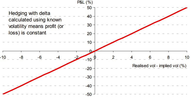
In a Black-Scholes world, the volatility of a stock is constant and known. As the position is initially delta-neutral (i.e., delta is zero), the gamma (or convexity) of the position generates a profit for both downward and upward movements. Although this effect is consistently profitable, the position does lose time value (due to theta). If an option is priced using the actual fixed constant volatility of the stock, these two effects balance each other out, and the position does not earn an abnormal profit or loss as the return equals the risk-free rate (theta pays for gamma).

The profit from delta hedging is equal to the difference between the actual price and the theoretical price. If an option is purchased at an implied volatility lower than the realized volatility, the difference between the theoretical price and the actual price will equal the profit of the trade. The relationship between profit and the difference in implied and realized volatility is direct. As theta and gamma are correlated, profits are not path dependent when hedged with the delta implied by the true volatility.

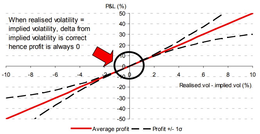
In reality, it's impossible to know the future volatility of a security in advance. As a result, one may use implied volatility to calculate deltas. However, delta hedging using this estimate introduces risk to the position, making it path dependent. Although the expected profit remains unchanged, the actual profits from delta hedging are no longer independent of the direction in which the underlying moves. This path dependency arises from the discrepancy between the correct delta (calculated using the remaining volatility to be realized over the life of the option) and the delta calculated using the implied volatility.

When there's a difference between the actual delta and estimated delta, there is risk, but not enough to make a cheap option unprofitable (or an expensive option profitable) as long as hedging is continuous. This is because in each infinitesimally small amount of time, a cheap option will always reveal a profit from delta hedging (net of theta), although the magnitude of this profit is uncertain. The extent of potential variation in profit is related to the difference between implied and realized volatility; a greater difference leads to an increased potential range of outcomes.

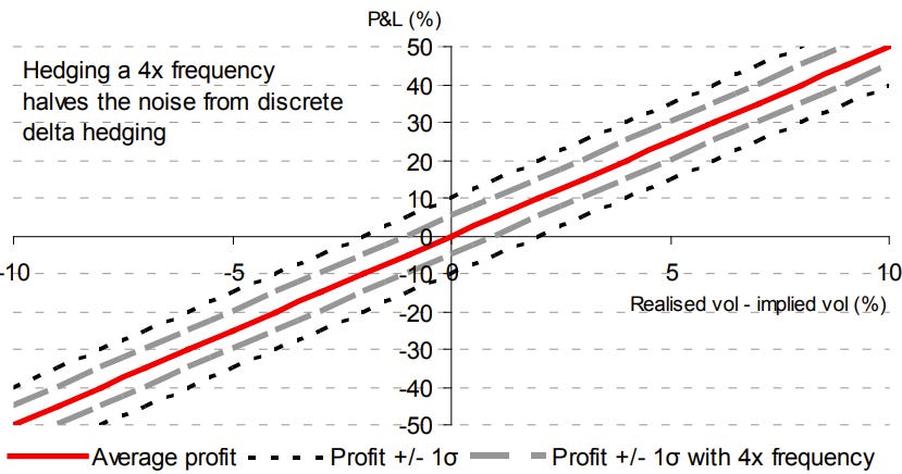
Discrete delta hedging with known volatility is a practical necessity, as continuous hedging is impossible due to trading costs, minimum trading sizes, limited trading hours, and non-trading periods like weekends. The accuracy of discrete hedging improves with increased frequency, with returns approaching those of continuous hedging in an ideal scenario of 24-hour trading and infinitely frequent hedging.

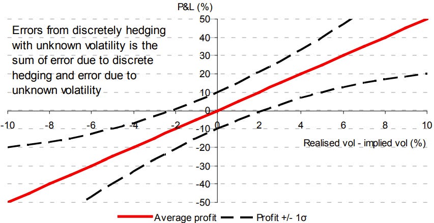
Importantly, hedging error is independent of average trade profitability. With known volatility, delta calculation errors are eliminated, and the introduced variation is essentially noise. This independence means that, unlike in continuous hedging where it's impossible to lose money on a cheap option, discrete hedging allows for potential losses on cheap options and gains on expensive ones.

The most realistic scenario for assessing profitability in options trading combines discrete delta hedging with unknown volatility. The two primary sources of variation in profit or loss are now combined: the inherent variation from discrete (rather than continuous) hedging, and the potential inaccuracy of the calculated delta due to unknown future volatility.

A paper by Ahmad and Wilmott gives the formula for PnL under different hedging schemes under slightly loosened Black-Scholes assumptions. Where V(a) is the value of the option under the actual realized volatility and V(i) is the value of the option under implied volatility, the lifetime PnL for hedging with the real vol is

\(e^{r t_0} \int_T^{t_0} d (e^{-rt}(V_i - V_a)) = V_a - V_i\)

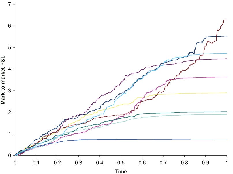
The final PnL is in theory not path dependent. The small discrepancies in the final PnL are due to discrete hedging in the simulation

As previously noted, if we hedge with implied vol, then profits are path dependent but buying a cheap option will always net a positive profit. The PnL is given by

\(2(\sigma^2 - \tilde{\sigma}^2) \int_{t_0}^T e^{-r(t-t_0)} S^2 \Gamma _i dt\)

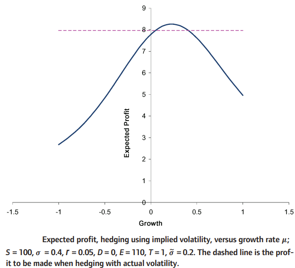
Is there some characteristic to the “optimal” path that gives us the most profit when we hedge with implied vol while still assuming geometric Brownian motion? The answer is yes. We know that gamma peaks at the money as expiration comes near, and so to maximize gamma exposure the expected profit is maximized roughly at the growth rate that ensures that the stock ends up close to at the money at expiration.

Hedging Error & Hedging Frequency

We now give some intuition to an approximation of gamma PnL variance as a function of hedging frequency. Recall that Gamma PnL for a hedged position over n periods can be given by the term

\(\frac{1}{2}\Gamma\epsilon_1^2 + \frac{1}{2}\Gamma\epsilon_2^2 + ... + \frac{1}{2}\Gamma\epsilon_n^2\)

The gamma PnL for an unhedged position can be given by

\(\frac{1}{2}\Gamma\ (\epsilon_1 + \epsilon_2 + ... + \epsilon_n)^2\)

Where epsilon represents small moves in the price of the underlying such that gamma can be assumed to be constant during that move. If we assume that excess returns of the underlying are normally distributed with zero mean and variance sigma, we can extract those variables and instead write the above two terms as

\(\frac{1}{2}\Gamma S^2 \sigma^2 \sum_{i=1}^{n}{x_i^2}, \ \ \ \text{and} \ \ \ \frac{1}{2}\Gamma S^2 \sigma^2 \left( \sum_{i=1}^{n}{x_i} \right)^2\)

where the xi terms are drawn iid from the standard / unit normal distribution with zero mean and variance of 1. It follows that the square of xi for any i is drawn from the Chi-squared distribution with one degree of freedom by definition. We can check that these two terms have the same expectation since

\(\left( \sum_{i=1}^{n}{x_i} \right)^2 = \sum_{i=1}^{n}{x_i} + \sum_{j=1}^{n} \sum_{i=1}^{j-1} x_i x_j\)

For each i not equal to j, the expectation of their production is 0 since the terms are drawn iid. To compare their variances, it is sufficient to compare the sum of squares versus the square of the sum. The sum of squares is trivial; for the square of the sum we define X to be equal to the sum from x1 to xn. Then, we note that

\(\mathrm{Var}[X^2] = \mathrm{E}[X^4] - \mathrm{E}[X^2]^2 = \mathrm{E}[X^4] - (\mathrm{Var}[X] + \mathrm{E}[X]^2)^2 \)

By the zero mean and unit variance of the xi terms we can write

\(\mathrm{Var}[X^2] = \mathrm{E}[X^4] - (n\mathrm{Var}[X_1] + 0)^2 = \mathrm{E}[X^4] - n^2\)

For the fourth moment of the sum X, we have

\(\begin{align*} \mathbb{E}[X^4] &= \sum_{i,j,k,l} \mathbb{E}[X_i X_j X_k X_l]. \end{align*} \)

We make the crucial observatio that if even one index is different from all the others then the term vanishes by zero mean. So removing all such terms from the summation, any surviving term must satisfy that for each index i there is another index which has the same value as i. This means that either (1) all the indices are the same, or (2) that the indices pair up. There are n ways for all the indices to be the same. There is n choose 2 (equal to n(n-1)/2) ways for us to get a pair of indices, and 4 choose 2 (equal to 6) ways to arrange them in 4 spots. As such, we have

\(\mathbb{E}[X^4] = n \mathbb{E}[X_1^4] + 3n(n-1)\mathbb{E}[X_1^2]^2 =n \mathbb{E}[X_1^4] + 3n(n-1) \)

We now aim to determine the expectation of the 4th moment. We integrate the pdf of the unit normal distribution over the reals twice by parts

\(E[X^4]=\frac{\displaystyle\int x^4e^{-x^2/2}dx}{\displaystyle\int e^{-x^2/2}dx}=\frac{-x^3e^{-x^2/2}+3\displaystyle\int x^2e^{-x^2/2}dx}{\displaystyle\int e^{-x^2/2}dx}=\frac{-3xe^{-x^2/2}+3\displaystyle\int e^{-x^2/2}dx}{\displaystyle\int e^{-x^2/2}dx}\)

Note that the left term in the numerator of the last fraction vanishes when evaluated; the value of the moment is therefore 3. For normal distributions with non-unit variance the 4th central moment we can deduce to be 3σ⁴. In any case, our unhedged position has PnL variance proportional to

\(3n + 3n(n-1) -n^2 = 2n^2\)

Our hedged position has PnL variance proportional to

\(n(\mathrm{E}[x_i^4] - \mathrm{E}[x_i^2]^2) = n(3-1)=2n\)

For n > 1, we see that the hedge position has a smaller variance. The gap is proportional to n(n-1). Here we have two competing intuitions; on one hand, by inspecting the case of n = 2 we note that hedging 2x vs 1x during an interval reduces the variance of the gamma PnL by 1/n(n-1) = 1/2. Applying this argument recursively, we see that hedging 4x as often brings down the standard deviation by 1/2.

On the other hand, we may be tempted to use the fact that n(n-1) is asymptotically n squared; for this case at least, it is more appropriate to use the first intuition. The idea that gamma PnL volatility is inversely proportional to the square root of hedging frequency also accords with the intuition that diffusion of price is proportional to the square root of time. Lastly, we note that hedging error accumulates linearly with respect to the number of hedging periods if frequency is held constant i.e. it accumulates linearly with respect to time but is inverse to the square root of frequency (a proof can be found in the appendix of Ed Thorp’s 1976 paper). So

\(\sigma_{PnL} \propto \frac{1}{2} S^2 \sigma^2 (T-t) \Gamma \sqrt{\frac{1}{N}}\)

Page 95 of Trading Volatility claims, without proof, that the normalization coefficient for this to become an equation is the square root of pi; if any reader can bother to find / figure out the proof for this I’d be happy to see it in the comments.

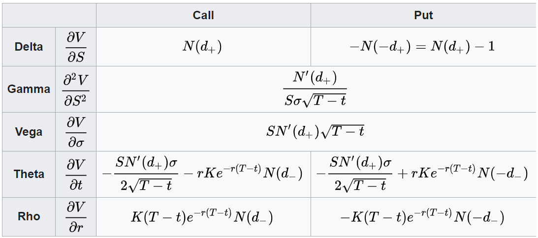
We can also replace Gamma with Vega for a more interpretable formula; from above we see that Vega is spot squared times vol times expiry times Gamma. This gives

\(\sigma_{PnL} = \text{Vega} \ \sigma\sqrt{\frac{\pi}{4N}}\)

Disclaimer

The information provided on TheLogbook (the "Substack") is strictly for informational and educational purposes only and should not be considered as investment or financial advice. The author is not a licensed financial advisor or tax professional and is not offering any professional services through this Substack. Investing in financial markets involves substantial risk, including possible loss of principal. Past performance is not indicative of future results. The author makes no representations or warranties about the completeness, accuracy, reliability, suitability, or availability of the information provided.

This Substack may contain links to external websites not affiliated with the author, and the accuracy of information on these sites is not guaranteed. Nothing contained in this Substack constitutes a solicitation, recommendation, endorsement, or offer to buy or sell any securities or other financial instruments. Always seek the advice of a qualified financial advisor before making any investment decisions.