

Implied Correlation and Index Skew
A Gentle Introduction to Dispersion Trades

Dispersion trading capitalizes on the relationship between the volatility of an index and the volatilities of its underlying components. An index’s implied volatility is determined by the volatilities of its constituent stocks and the degree to which these stocks move together, i.e. their correlation. When the components are highly correlated, the index volatility tends to align closely with the average volatility of its components. Conversely, if the correlations are low, the index volatility will generally be lower than the volatilities of its individual stocks.
Dispersion & Implied Correlation
Suppose we have 10 stocks, each with weight
Let Ri be the (random) return of stock i. The index return is then
Denote the volatility of stock i by σi, and the correlation between stocks i and j by ρij. The variance of the index is then
For simplicity, if we assume a constant correlation across all pairs of stocks and constant volatility for each stock. Then the index variance simplifies to
In reality, volatilities and correlations differ across stocks (in which case the implied corr is roughly the index var divided by a weighted average of stock var); however, the above equation shows the correct intuition that the index variance is roughly proportional to the product between individual stock average variance and the average correlation between the underlying index components (for small changes).
What does it Mean to Trade the Dispersion?
Single-stock volatility and index volatility are both directly observable in the market—each stock has an implied volatility quoted on its individual options, and an index has its own implied volatility derived from index options. At the same time, both single-stock and index volatility can be observed in realized form through historical returns.
In contrast, pairwise correlation (i.e., the correlation between specific pairs of stocks) is only truly observable in realized form by examining how those two stocks have co-moved historically; there is no separate, widely tradable “pairwise correlation” option market. Instead, what is more readily traded (and thus can be implied from option prices) is an “average correlation” that summarizes how a basket of constituents behaves as a whole—most notably inferred by comparing the index’s implied volatility to the weighted combination of its constituents’ implied volatilities.
This average correlation, therefore, exists both in realized space (computed from historical index and constituent movements) and in implied space (backed out from index and single-name option prices). Because it can be extracted from option markets, average correlation is more directly tradable through strategies such as dispersion trading, whereas true pairwise correlation among two individual stocks remains hard to trade without access to structured products.
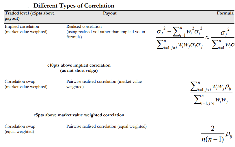
Per Trading Volatility page 166, the profit from an options-constructed dispersion is roughly the difference between implied and realized correlation multiplied by the average single-stock volatility. As correlation is correlated to volatility, this means the payout when correlation is high is increased (as volatility is high) and the payout when correlation is low is decreased (as volatility is low). A short correlation position from going long dispersion (short index variance, long single-stock variance) will suffer from this as profits are less than expected and losses are greater.
Dispersion is therefore short vol of vol; hence, implied correlation tends to trade above levels implied by correlation swaps (which is a more pure expression of correlation, that itself trades above realized correlation). We note this does not necessarily mean a long dispersion trade should be profitable (as dispersion is short volga, the fair price of implied correlation is above average realized correlation).
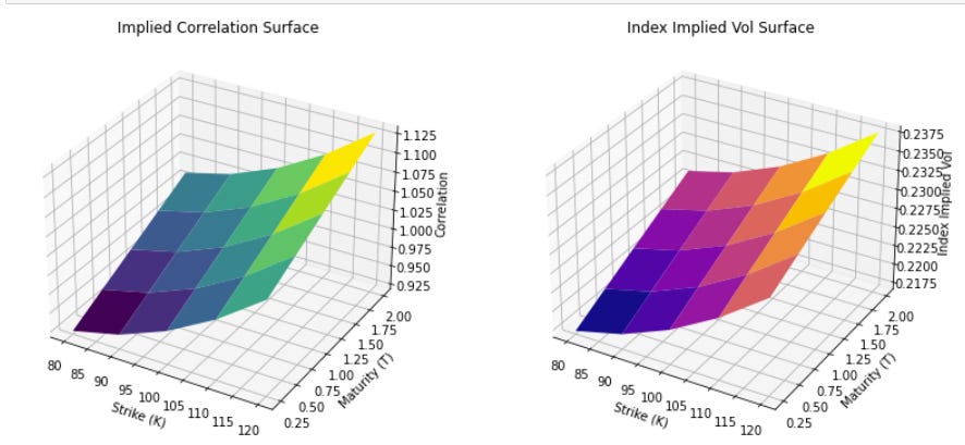
The Implied Correlation Surface
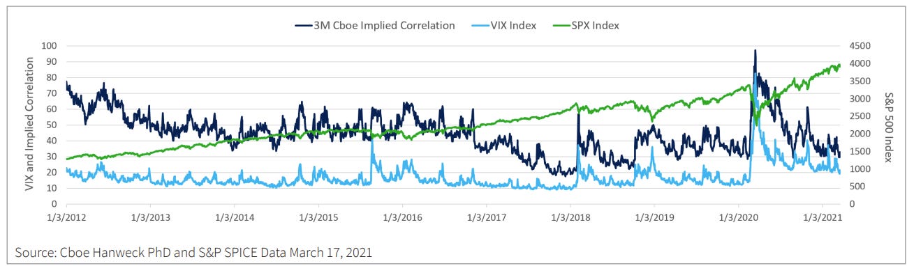
CBOE facilitates the trading of correlation indices (they market it as the market expectation of the benefits of diversification). While there are 500 members of the S&P 500, the CBOE calculation only takes the top 50 stocks (to ensure liquidity); the full methodology can be found here. We can plot the implied correlation over time along with the S&P 500 and the VIX to see that correlations spike when vol does.
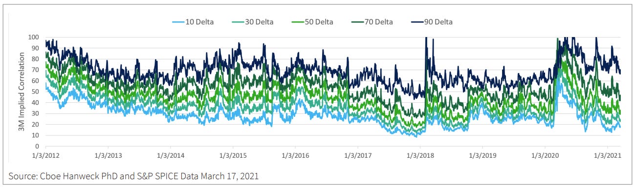
Another interesting fact about the implied correlation surface is that it is skewed. We expect this intuitively since discrepancies between single-stock skew and index skew inevitably must be accounted for by skew in implied correlation space (otherwise there will be arb). If single-name options display a mild put skew (or even a call skew in some cases) while index options exhibit a pronounced put skew, then the index skew must be reconciled via higher implied correlation on the downside in order to align the pricing of index puts with the aggregated pricing of constituent puts.
Implied Correlation and Index Skew
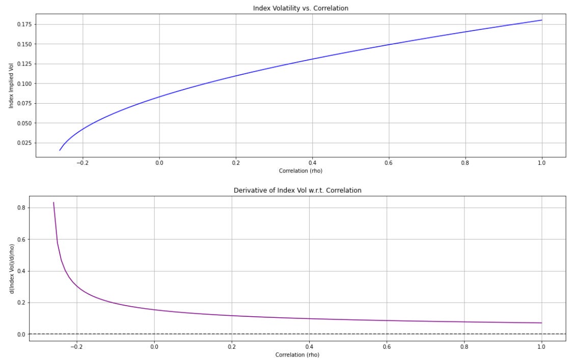
We note that the partial derivative of index vol with respect to correlation is concave. I.e. moving correlation from negative values to zero or mildly positive produces a large jump in the index volatility — reducing the benefits of diversification greatly — but moving correlation from, say, 0.8 to 0.9 does not cause as big a difference. We can show this mathematically below
Denote the terms
Then we can simply write
The partial derivative of index vol with respect to correlation is then
Which we see is diminishing on the order of 1/sqrt(corr). This might seem counterintuitive to some: one might expect that going from already-high correlation to even higher correlation would have a major effect. Yet, when portfolios move from negative correlation (or zero correlation) to even modest positive correlation, the marginal loss of diversification is large. That early “shock” of going from offsetting or unrelated assets to correlated assets hammers portfolio diversification benefits. In contrast, going from already-high correlation (e.g., 0.8) to an even higher number (e.g., 0.9) still means stocks are moving in near lockstep—so the incremental effect on index vol is smaller. This ties in with the common portfolio management principle that adding even a lower-Sharpe, but negatively or uncorrelated asset, can significantly improve the overall Sharpe ratio, whereas tacking on yet another positively correlated asset adds far less incremental diversification benefit.
A related “brain teaser” question is: What happens to index skew if we raise the entire implied correlation surface uniformly by one point?
At first glance, some might guess that higher correlation universally implies a steeper index skew, because in crises we expect correlation to spike. However, due to the concavity of the correlation–volatility relationship, the effect on index vol at strikes where implied vol is already high (i.e., deep puts) is relatively smaller compared to the effect at strikes where implied vol is lower (near or above the money). Consequently, the actual outcome can be that the index skew flattens rather than steepens. The incremental jump in volatility for those higher-vol, deep-put strikes is smaller (they’re already in a “high correlation” regime), while for the near-the-money or call strikes, which started with lower correlation assumptions, the jump in implied vol can be larger. Hence, uniform upward shifts in the correlation surface may end up reducing the slope of the index skew curve rather than increasing it.
Disclaimer
The information provided on TheLogbook (the "Substack") is strictly for informational and educational purposes only and should not be considered as investment or financial advice. The author is not a licensed financial advisor or tax professional and is not offering any professional services through this Substack. Investing in financial markets involves substantial risk, including possible loss of principal. Past performance is not indicative of future results. The author makes no representations or warranties about the completeness, accuracy, reliability, suitability, or availability of the information provided.
This Substack may contain links to external websites not affiliated with the author, and the accuracy of information on these sites is not guaranteed. Nothing contained in this Substack constitutes a solicitation, recommendation, endorsement, or offer to buy or sell any securities or other financial instruments. Always seek the advice of a qualified financial advisor before making any investment decisions.
Are the correlation skew indices computed using implied volatilities based on specific moneyness or do they determine a volatility surface and then "read" the volatility at a specific moneyness?
Very interesting brain teaser, so short SPX skew is somewhat long correlation?