
Multidimensional Greeks
Introduced with Rainbow Options

Visuals and some content taken from page 387 to 389 of Dynamic Hedging
When we first encounter options Greeks, they are typically introduced in the context of a single underlying asset. Each Greek measures sensitivity to a particular parameter: Delta for price, Vega for volatility, Theta for time, and so on. These are essentially one-dimensional concepts—each Greek is a scalar. However, just as single-variable calculus evolves into multivariable calculus, the mathematics of derivatives naturally extends when we move from vanilla options to multi-asset derivatives.
In particular, consider a rainbow option defined by one expiration date and a payoff that is equivalent to the largest in the money portion of any of the strike prices. For example, a rainbow call over n assets has terminal value
In the simple case with assets, we can visualize the payoff
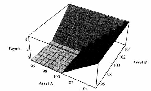
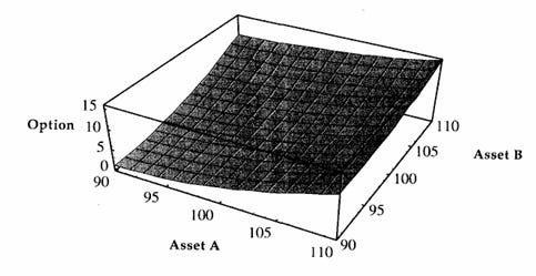
Prior to expiration, the value of the option will be strictly above this payoff with the highest difference achieved at (100, 100).
We can intuitively see that the final payoff above covers more area than either of the two options taken separately but less than the sum of two independent options.
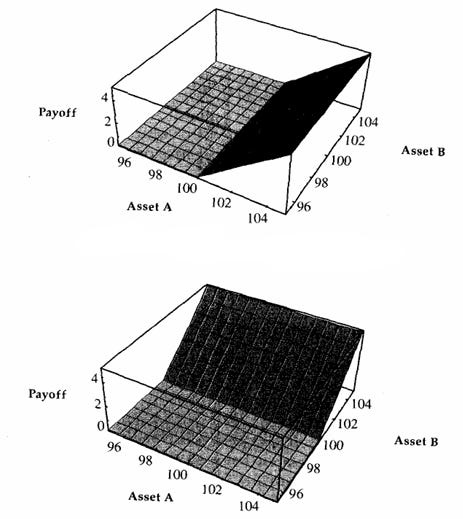
The value of the difference between the two independent options and the rainbow is captured by the correlation between the underlying assets. Assuming both assets are ATM with the same price, strike, and volatility, then at correlation 1 it no longer matters that there is a second asset, and the rainbow will trade at the price of either one of the individual options (both have the same price).
At correlation -1 the rainbow trades at exactly 2x the price of the individual options, this is since for each up move in one asset, the other will move down by the exact same amount, and vice versa; the rainbow is therefore equivalent to a straddle as one asset will always be ITM given small perturbations. At 16 vol T = 1 and S = 100 for both assets, we have the following graph showing the price of the option vs. corr
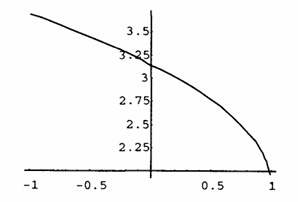
Similarly, we note that a rainbow option that has a call on one asset and a put on another asset would have an inverse relationship to correlation compared to a rainbow option that uses two calls or two puts.
The “volatility” of the structure is naturally represented by the covariance matrix, as variance is is naturally extended to covariance
By inspection, the covariance matrix admits the decomposition
I.e. the covariance matrix decomposes into the product between diagonal matrices with the volatilities and a symmetric matrix with the correlations. That this decomposition is always possible follows from the fact that a covariance matrix is always symmetric and positive semidefinite. In particular, symmetry follows from the definition of covariance and positive semidefiniteness follows from the fact that any weighted combination of the variables will have non-negative variance. The spectral theorem from linear algebra tells us that any symmetric matrix can be diagonalized into a product of eigenvectors and eigenvalues. By the Gram-Schmidt process a change of basis from the eigenvectors back to the original vectors; i.e. the original covariance structure is fully recoverable from the spectral decomposition.
In the context of multi-asset options, the above decomposition naturally leads to the idea of a correlation Vega. I.e. because the joint distribution of asset returns influences the probability of various payoff scenarios, the correlation between assets becomes a risk factor in itself, and the correlation Vega represents that risk.
Moving on, the delta of the structure is naturally represented by a gradient
Where each entry in the gradient is best described as a partial delta. The gradient has a natural interpretation which is that it is the sensitivity of the structure to the prices of either A or B assuming that they move according to their correlation. I.e. we assume that price movements are along a vector that points in the direction of the steepest ascent (or greatest rate of increase) of the option’s value surface at that point.
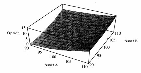
The relationship between the partial delta and gradient is shown below with 0.5 corr
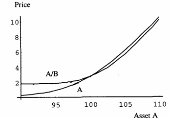
The gradient is therefore best interpreted as a “correlated” delta; the “uncorrelated” delta is best represented as the total derivative
The above result shows that you're long Delta in multiple assets, and those assets are highly correlated, the portfolio can behave as though it's exposed to a single large position; but if the assets are uncorrelated (or negatively correlated), the combined Delta risk can “diversify” and you need to hedge less in either asset to be delta-flat.
The idea of partial and total deltas naturally lead to the notion of partial gamma. In particular, for the 2-asset rainbow there are four partial gammas
Where Gamma AA denote changes in Delta A stemming from changes in A’s price (assuming B moves by its correlation), Gamma AB denotes changes in Delta A stemming from changes in B (assuming A moves by its correlation), etc…
The idea of multi-dimensional Greeks naturally leads to the notion of a multi-asset Black-Scholes framework, which while mathematically rich, is also quite involved.
But even without diving deep into the equations, the structure we've built so far provides a strong intuitive foundation for understanding the key risk sensitivities for multi-asset options. Correlated Delta risk can be thought of either as a gradient—a vector of sensitivities to each asset—or as a total derivative. Volatility can be seen as encapsulated by a covariance matrix, and as such correlated Vega risk naturally splits into separate sensitivities to each asset’s volatility and to their mutual correlation, reflecting how both marginal and joint uncertainty affect option value. Gamma becomes richer too—it now captures how the Delta with respect to one asset changes when any of the assets move, not just that asset alone.
The reader may feel that theory regarding options whose payoff depends on multiple underlying assets is an exotic corner of financial theory that while mathematically elegant, is ultimately not useful. But one of the most important and liquid contracts in the world, the Treasury futures contract, can in fact be interpreted as a multi-underlying option.
In this case the short party (the seller) has the right to deliver any bond from a set of eligible securities. This means the short effectively holds an option to deliver the cheapest-to-deliver (CTD) bond from a basket—i.e., they choose the bond that minimizes their delivery cost. There is therefore an embedded rainbow put option on a set of bonds (or a put-on-minimum outperformance option) assuming that rates can’t go below 0. This structure, while embedded and not priced as an explicit option, reveals how option theory can be used in the pricing of interest rate products (or indeed, any product) with embedded optionality.
Disclaimer
The information provided on TheLogbook (the "Substack") is strictly for informational and educational purposes only and should not be considered as investment or financial advice. The author is not a licensed financial advisor or tax professional and is not offering any professional services through this Substack. Investing in financial markets involves substantial risk, including possible loss of principal. Past performance is not indicative of future results. The author makes no representations or warranties about the completeness, accuracy, reliability, suitability, or availability of the information provided.
This Substack may contain links to external websites not affiliated with the author, and the accuracy of information on these sites is not guaranteed. Nothing contained in this Substack constitutes a solicitation, recommendation, endorsement, or offer to buy or sell any securities or other financial instruments. Always seek the advice of a qualified financial advisor before making any investment decisions.