Options Implied Distributions are NOT Real-World Distributions

Risk-Neutral Measures vs Physical Measures

There is sometimes a misunderstanding, even among practitioners, that option prices reflect the market’s view of the distribution of an asset’s price at expiry. This emerges out of a serious misunderstanding of the difference between the risk neutral measure used to price derivatives in complete markets and the real world measure which determines the actual distribution of asset prices. We will try not to dive too deep into the math in this post (probably just give proof outlines and statements of the main theorems used) but a good understanding of probability and options theory (academic, not practical) may be helpful.

Introduction

This post is dense; the following roadmap gives the major themes and logical flow:

1. Construction of “Implied Probabilities.” Shows how tight butterfly spreads and interpolated volatility surfaces yield a risk-neutral distribution.

2. Disappearance of Drift. Demonstrates via delta-hedging that the stock’s real-world drift μ vanishes from the valuation PDE, leaving only the risk-free rate r.

3. Fundamental Theorem & Arrow–Debreu. Links no-arbitrage and market completeness to the existence and uniqueness of a single risk-neutral (Q) measure, with state prices backing out both CAPM and arbitrage-pricing models.

4. Feynman–Kac & Change of Measure. Applies the Feynman–Kac formula and Girsanov’s theorem to show how the stochastic discount factor—aka the intertemporal marginal rate of substitution—reweights P into Q.

5. Deflation of Price Distribution. Quantifies how compounding at μ > r inflates absolute price deviations under P, so that Q-based probabilities exaggerate downside risk (volatility skew).

6. Positive-EV Option Trades. Examines how collars or deep-OTM put sales exploit the Q–P gap—and explains why, under CAPM equilibrium, no option strategy can out-Sharpe a leveraged market portfolio.

7. When Implied Views Align with Reality. Identifies circumstances (short maturities, earnings windows, incomplete markets) where option-implied distributions approximate true probabilities.

How Options Implied Probabilities Are Calculated

Exposure to a specific range of stock price outcomes can be acquired with a butterfly spread (long 1 low strike call, short 2 higher strikes calls, and long 1 call at an even higher strike). The “probability” of the stock ending in that range is then calculated as the cost of the butterfly, divided by the payout if the stock is in the range. The payoff for the butterfly is shown below

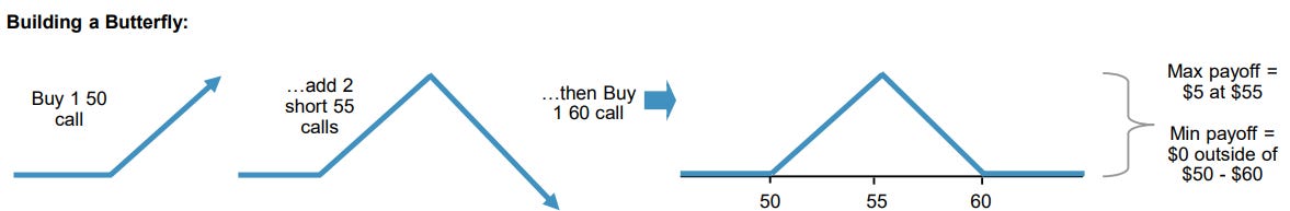
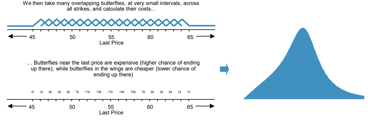
To extrapolate a probability distribution, we can first extrapolate an implied volatility surface from observable discrete market strikes, and then price a series of theoretical call options at various strikes (which can now be arbitrarily close) using the interpolated volatility surface. With these calls we can price a series of very tight overlapping butterfly spreads; dividing the costs of these trades by their payoffs, and adjusting for the time value of money, yields the “implied probability distribution” of the stock as priced by the options market

In the following sections of this post, we will discuss why using options implied probability to estimate future stock prices often yields a distribution with expected returns and perceived risk significantly lower than the market's actual expectations.

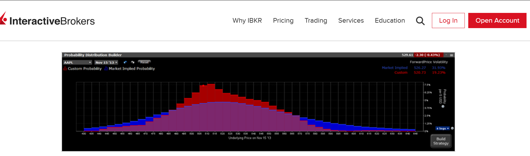
For brokerage firms this characteristic of option-implied distributions can be strategically advantageous. By presenting the options market as underpricing the expected return of stocks brokers can potentially attract more retail investors from whom they can collect additional fees. For example, IBKR Probability Lab allows retail traders to view the market implied distribution, and to determine the “optimal” trades based on the differences between the trader’s view and the market’s view

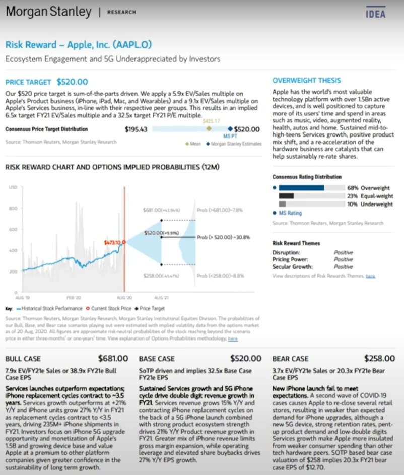
Similarly, S&T teams might benefit from employing these distributions to appeal to clients by portraying the risks associated with certain stocks / investments as less severe than they actually are. This can lead clients to invest more heavily or venture into asset classes they might otherwise consider too risky, under the belief that the market conditions are more benign than they actually are. For example, consider the following report from Morgan Stanley Equity Research on AAPL

In order to discuss with some level of rigor why the above practices are problematic, we will need to first clear up some terminology. In particular, our discussion will be about how the risk-neutral measure differs from the physical market measure, and as such we will first need to understand what a “measure” is and what “market” is.

What is a Probability Measure?

The Wikipedia definition for a probability measure is characteristically unhelpful “In mathematics, a probability measure is a real-valued function defined on a set of events in a σ-algebra that satisfies measure properties.” We will instead try to give an intuitive definition of the terminology using the example of flipping a fair coin. Recall that a probability space consists of:

1. A sample space X, which is the set of all possible outcomes

2. A collection of events Σ, which are subsets of X

3. A function μ, called a probability measure, that assigns to each event in Σ a nonnegative real number

In the case of flipping a fair coin, we have

\(X=\{H,T\}\)

\(\Sigma=\{\varnothing,\{H\},\{T\},X\} \)

\(\mu(\varnothing)=0, \mu(\{H\})=\mu(\{T\})=\frac{1}{2},\mu(X)=1 \)

All of this to say that when I flip a coin, I have a 0 percent chance of flipping nothing, a 50 percent chance of flipping heads, a 50 percent chance of flipping tails, and a 100 percent chance of flipping something. This is all very intuitive.

There are certain natural requirements that Σ and μ must satisfy. For example, it is natural to require that ∅ and X are elements of Σ, that μ(∅) = 0, and that μ(X) = 1 (i.e. when performing an experiment, the probability that no outcome occurs is 0, while the probability that some outcome occurs is 1). There are other requirements of μ which make it a (finite) measure, but in essence a measure is simply a function that assigns to each event in Σ a nonnegative real number.

Similarly, it is natural that there are some requirements we think Σ should have in relation to μ (note that the prior constraints on μ were independent of Σ). For example, if E ∈ Σ is an event, then μ(Eᶜ) + μ(E) = 1 (i.e. when performing an experiment, the probability that event E occurs or doesn’t occur must be 1). There are, of course, other requirements of Σ which make it a σ-algebra, but in essence a σ-algebra is just a set of events that satisfies very reasonable logical constraints.

Regarding market measures, the sample space encompasses all potential outcomes for a given financial variable, such as the set of all possible price levels a stock might reach over a specified period. Within this framework, events represent specific outcomes or collections of outcomes within the sample space that are of interest, such as a stock price exceeding a particular value at a future date. The two principal measures that typically arise in the academic discussion are the risk-neutral measure and the physical measure, which is also the topic of our post.

Risk-Neutral Measure (Q-measure): Probabilities under the risk-neutral measure are assigned assuming all investors are risk-neutral (they do not demand extra returns for bearing additional risk). Therefore, the expected returns of assets are discounted at the risk-free rate, regardless of their risk. This is a mathematical construct.

Physical Measure (P-measure): Probabilities under the physical measure are based on actual investor expectations and behaviors, accounting for risk preferences and other market forces. These probabilities forecast actual outcomes but are unobservable.

It cannot be stressed enough that the risk-neutral measure constructs a theoretical world where all investors are risk-neutral, whereas the physical measure reflects the actual behaviors and expectations of market participants. Thought of another way, the risk-neutral measure adjusts the probabilities of future states of the world so that the expected return of all assets becomes the risk-free rate when discounted back to the present. This adjustment can be seen as a transformation of the original random variables (representing asset prices or returns under the real-world measure) into new random variables that reflect the market’s collective expectations under the assumption of risk neutrality.

The Drift Term Disappears in Derivative Pricing

Assume that the stock price S(t) follows a Geometric Brownian Motion (i.e. the stochastic process it would follow if returns were iid normally distributed) under the real world physical measure P

\(\frac{dS_t}{S_t} = \mu dt + \sigma dW_t^{\mathbb{P}}\)

where μ is the expected performance of the stock and σ the annualized volatility of log-returns. Consider the pricing (we are still in the real world) of ANY contingent claim

\(V_t = V(t,S_t) \)

of which the only thing we know is that it pays out ϕ(ST) to its holder when t=T (generic European option). Now, consider the following self-financing portfolio

\(\Pi_t = V_t - \alpha S_t \)

Using Itô's lemma along with the self-financing property

\(\begin{align} d\Pi_t &= dV_t - \alpha dS_t \\ &= \left( \frac{\partial V}{\partial t} + \frac{1}{2} \sigma^2 S_t^2 \frac{\partial^2 V}{\partial S^2}\right) dt + \left( \frac{\partial V}{\partial S} - \alpha \right) dS_t\\ \end{align}\)

The original argument of Black, Scholes, and Merton is then that if we can dynamically rebalance the portfolio Πt so that the number of shares held is continuously adjusted to be equal to α=∂V/∂S (this is called delta hedging), then the portfolio Πt would drift at a deterministic rate which, by absence of arbitrage, should match the risk-free rate. Therefore, it follows that

\(\begin{align} &d\Pi_t = \Pi_t r dt \\ \iff& \left( \frac{\partial V}{\partial t} + \frac{1}{2} \sigma^2 S_t^2 \frac{\partial^2 V}{\partial S^2} \sigma^2 \right) dt = \left( V_t - \frac{\partial V}{\partial S} S_t \right) r dt \\ \iff& \frac{\partial V}{\partial t}(t,S) + r S \frac{\partial V}{\partial S}(t,S) + \frac{1}{2} \sigma^2 S^2 \frac{\partial^2 V}{\partial S^2}(t,S) - rV(t,S) = 0 \end{align}\)

which is of course the Black-Scholes equation.

Properties of the Risk-Neutral Measure

We can now start to answer why options (and indeed, all derivatives) should be priced using the risk-neutral measure while the underlying assets themselves follow the physical measure. It turns out that, using a replication argument (static for linear contracts, dynamic for others) and under the assumptions of no arbitrage, market completeness, continuous trading, and no frictions, one can show that the true performance of the stock μ simply disappears from the option‐valuation problem (as shown above) and only the risk-free rate r remains; i.e., an option (or indeed, any contingent claim/derivative) can be manufactured using dynamic hedging of the underlying, and its value evolves according to the Black–Scholes stochastic PDE.

Intuitively, the fact that all self‐financing portfolios composed of a derivative and dynamically or statically hedged with marketed securities must grow at the risk-free rate means that we can price these derivatives as if the underlying grows at the risk-free rate (and can skip the math of solving the PDE for the particular boundary conditions associated with different contingent claims). Why? Consider the case of a forward contract (probably the simplest contingent claim), where the risk-free position is constructed by selling the forward and buying the stock now; note that the same valuation can be reached by assuming that the stock drifted at the risk-free rate. However, the fact that a 10-year forward can be sold on the SPX index with the risk-free forward rate doesn’t actually mean that anyone expects U.S. large-cap stocks to return the risk-free rate for the next 10 years; instead, it demonstrates the difference between the risk-neutral and physical measures.

The above argument may not be totally convincing; in particular, we need to show that the risk-neutral measure is the unique measure that, when used on the underlying, allows all contingent claims to satisfy the Black–Scholes stochastic PDE (under certain regularity conditions). The proof for this claim is pretty mathematically involved (so we offer only an outline); two main results we will need are:

1. Fundamental Theorem of Asset Pricing: The condition of no-arbitrage is equivalent to the existence of a risk-neutral measure.

2. Law of One Price: Completeness of the market is equivalent to the uniqueness of the risk-neutral measure.

Measure Construction using Feynman–Kac

Now, we note that the Black–Scholes PDE is a parabolic PDE and apply the Feynman–Kac formula from physics. Intuitively, this formula establishes a link between parabolic partial differential equations and stochastic processes, essentially allowing us to solve the PDE by simulating random paths of a related stochastic process; i.e., the PDE describes the flow of a time-dependent probability distribution, and the stochastic process describes individual realizations (random walks with a drift)—but if we ran a large number of them, we’d build up the same distribution.

It is easy to see why transforming PDEs into stochastic processes is useful in physics. For example, one can express particles’ behaviors as averages over all possible paths they could take, weighted by their quantum-mechanical probabilities. In any case, the formal statement of the theorem is that given the PDE

\({\displaystyle {\frac {\partial }{\partial t}}u(x,t)+\mu (x,t){\frac {\partial }{\partial x}}u(x,t)+{\tfrac {1}{2}}\sigma ^{2}(x,t){\frac {\partial ^{2}}{\partial x^{2}}}u(x,t)-V(x,t)u(x,t)+f(x,t)=0}\)

defined for all x∈R and t∈[0,T] subject to the terminal condition

\(u(x,T)=\psi (x)\)

where μ, σ, ψ, V, f are known functions, T is a parameter, and u is the unknown. Then the Feynman–Kac formula expresses u(x,t) as a conditional expectation under the probability measure Q

\({\displaystyle u(x,t)=E^{Q}\left[e^{-\int _{t}^{T}V(X_{\tau },\tau )\,\mathrm {d} \tau }\psi (X_{T})+\int _{t}^{T}e^{-\int _{t}^{\tau }V(X_{s},s)\,\mathrm {d} s}f(X_{\tau },\tau )\,\mathrm {d} \tau \,{\Bigg |}\,X_{t}=x\right]}\)

Where X is an Itô process satisfying

\({\displaystyle \mathrm {d} X_{t}=\mu (X_{t},t)\,\mathrm {d} t+\sigma (X_{t},t)\,\mathrm {d} W_{t}^{Q}}\)

and W is Brownian motion under Q. The physics interpretation (per Wikipedia) is to consider the position X(t) of a particle that evolves according to the diffusion process given above, and let the particle incur "cost" at a rate of f(Xs,s) at location Xs at time s and a final cost at ψ(XT) while also allowing the particle to decay such that if the particle is at location Xs at time s, then it decays with rate V(Xs,s) and after the particle has decayed, all future cost is zero; then u(x,t) is the expected cost-to-go if the particle starts at (t,Xt=x). Applying Feynman-Kac directly on Black-Scholes gives

\(V_0 = E^\mathbb{Q}[ e^{-rT} \phi(S_T) \vert \mathcal{F}_0 ] \)

where under a certain measure Q

\(\frac{dS_t}{S_t} = r dt + \sigma dW_t^{\mathbb{Q}} \)

which is what we wanted to show (the drift rate under Q is indeed r).

Risk-Neutral Valuation is Consistent with General Equilibrium

Applying Feynman-Kac very much resembles a magic trick, and it is not immediately clear what is going on. Zooming in on the change of measure can perhaps be enlightening. The gist of the argument here is that we can define a quantity λ as the excess return over the risk-free rate of our stock (i.e. Sharpe ratio), which then gives the real world diffusion process

\(\frac{dS_t}{S_t} = r dt + \sigma (dW_t^{\mathbb{P}} + \lambda dt) \)

Using Girsanov theorem and manipulating the Radon-Nikodym derivative one can eventually show (you have to just take my word here) that

\(V_0 = E^{\mathbb{Q}} \left[ e^{-rT} \phi(S_T) \vert \mathcal{F}_0 \right] = E^{\mathbb{P}} \left[ e^{-\left(r+\frac{\lambda^2}{2}+\frac{\lambda}{T} W_T^{\mathbb{P}}\right)T} \phi(S_T) \vert \mathcal{F}_0 \right] \)

This shows that, under BS assumptions:

1. The option price can be calculated as an expectation under Q in which case we discount cash flows at the risk-free rate

2. The option price can also be calculated as an expectation under P but this time we need to discount cash flows based on our risk-aversion, which transpires through the market risk premium λ (which depends on μ)

Put in plain words, the price of an option should be the same for a holder who is delta-hedging (earning the risk-free rate) as for a holder who is not (exposed to potentially higher returns but also higher risk), assuming both are acting “rationally.”

The simplest example is the forward on the market portfolio: replication yields the risk-free rate (which lies on the Security Market Line of the CAPM, satisfying general equilibrium), while buying the forward outright gives leveraged exposure to the market portfolio (also on the SML). In that case, the expected return is higher but is discounted at a rate corresponding to its own return, so the forward’s present value still uses only the risk-free rate.

Under the real-world (physical) measure, asset prices depend crucially on their risk, since investors typically demand higher returns for bearing additional risk. Thus, today’s price of a claim on a risky payoff realized tomorrow will generally lie below its expected value, compensating those who bear the risk.

In a complete market with no arbitrage, every derivative can be replicated via dynamic hedging, which leads to a stochastic differential equation (the Black–Scholes PDE) governing all contingent-claim prices. For certain boundary conditions—those that define a claim’s payoff—we obtain closed-form solutions, though not in every case.

It turns out, however, that there exists a unique measure equivalent to the one under which all investors are risk-neutral. By adjusting the probabilities of future outcomes—that is, by switching to this new “risk-neutral” measure—we effectively embed all investors’ risk premia into derivative prices. Taking expectations under the risk-neutral distribution then produces the same valuations as solving Black–Scholes.

The Stochastic Discount Factor

We are now able to answer the question of what is the relationship between the risk-neutral measure and the physical measure? As demonstrated in the section above, if we assume a particular risk premium λ then we can show that the expectation under the risk-neutral measure is equal to the expectation under the physical measure discounted by some stochastic discount factor, copying from above we have

\(V_0 = E^{\mathbb{Q}} \left[ e^{-rT} \phi(S_T) \vert \mathcal{F}_0 \right] = E^{\mathbb{P}} \left[ e^{-\left(r+\frac{\lambda^2}{2}+\frac{\lambda}{T} W_T^{\mathbb{P}}\right)T} \phi(S_T) \vert \mathcal{F}_0 \right] \)

If we assume Black-Scholes assumptions to be true, estimating real-world probabilities becomes straightforward; the natural idea is to calibrate our diffusion model to observed time series; i.e. get an estimate for μ (risk-free returns plus risk premium) and σ (known constant volatility) in the GBM case. It's more interesting when we think about the general case though. In particular,

\(V_0 = E^{\mathbb{Q}} \left[ \frac{V_T}{B_T} \vert \mathcal{F}_0 \right] = E^{\mathbb{P}} \left[ \frac{V_T}{B_T} f \vert \mathcal{F}_0 \right], \ \ \ \ \ f = \left. \frac{d\mathbb{Q}}{d\mathbb{P}} \right\vert_{\mathcal{F}_T} \)

will hold (under mild regularity conditions). The risk-free discount factor and the Stochastic Discount Factor are each given by

\(DF (0,T):=1/B_T, \ \ \ \ \ SDF (0,T):=f/B_T \)

and so in the general case we have

\(V_0 = E^{\mathbb{Q}} \left[ DF (0,T) V_T \vert \mathcal{F}_0 \right] = E^{\mathbb{P}} \left[ SDF (0,T) V_T \vert \mathcal{F}_0 \right] \)

The problem is that, depending on the model assumptions we use, we may not have a closed-form for f as it was in Black-Scholes; e.g. for incomplete models (i.e. models that include jumps and/or stochastic volatility etc…).

We have now showed that SDFs emerge naturally from the existence of a risk-neutral measure, but it is perhaps even more enlightening to see the risk-neutral measure emerge naturally from the existence of SDFs. For this, we consider state-spaces

• Let X be a random variable denoting a risky cash flow next period

• Let f(X) be a pricing function which gives today's price for a risky cash flow

An obviously desirable feature of f is that it should be linear; if f is a linear function then one can show that there exists a stochastic discount factor M such that

\(f(X) = \operatorname{E}^\mathbb{P}[MX]\)

If we're in a discrete probability space with n possible outcomes (for simplicity), then for any linear functional f, there exists an M such that f can be written as

\(f(X) = \sum_i p_i m_i x_i \)

That whole M business is be rather inconvenient, we want to get rid of the SDF. Let

\(q_i = \frac{p_i m_i}{\sum_j p_j m_j} \)

Observe now that

\(\sum_i q_i = 1 \)

so that Q is a probability measure. Also observe that the risk free rate satisfies

\(1 = \sum_i p_i m_i (1 + r_f) \)

hence

\(\sum_i p_i m_i = \frac{1}{1 + r_f}\)

putting it all together

\(\operatorname{E}^\mathbb{P}[MX] = \sum_i p_i m_i x_i = \frac{1}{1+r_f} \sum_i q_i x_i = \frac{1}{1+r_f} \operatorname{E}^\mathbb{Q}[X] \)

Which again shows that for pricing, the following gives the same result

1. Probability measure P along with the stochastic discount factor M

2. A tilted probability measure Q and risk neutral pricing.

The essential idea here is that each state of the world i may have a different state prices and risk neutral pricing is a “trick” that for convenience, we can pack this into a tilted probability measure Q where q is proportional to p times m. What takes us back and forth between P (the physical measure) and Q (the risk-neutral measure) is the stochastic discount factor M. Essentially, this factor divides expected utility at the relevant future period - a function of the possible asset values realized under each state - by the utility due to today's wealth, and is then also referred to as the intertemporal marginal rate of substitution.

Hence (with the math above), we see that despite its name, the risk-neutral measure is actually affected by investors risk-aversion i.e. it is the physical measure that represents true probabilities. The risk-neutral measure incorporates the concept of risk aversion directly through the stochastic discount factor, which adjusts the real-world probabilities by discounting future cash flows at a rate that strips out the risk premiums. This adjustment is achieved mathematically using Girsanov’s theorem.

The implications of this transformation are nontrivial, particularly when interpreting the probabilities implied by option prices. In a risk-neutral world, the probabilities associated with different outcomes (such as the prices at which a stock might trade in the future) are adjusted to reflect a world where investors do not require risk compensation. This leads to a scenario where downside risks are often exaggerated compared to their real-world probabilities. The risk-neutral probabilities derived from options markets, therefore, should not be naively interpreted as the actual probabilities that real-world investors assign to these outcomes.

This exaggeration of downside risks is a direct result of risk aversion—investors are more concerned about potential losses than equivalent gains, leading to higher premiums for protection against downside movements. Options markets reflect this through higher implied volatilities for out-of-the-money put options compared to call options at the same distance from the current stock price, a phenomenon often observed as volatility skew.

The SDF and the Marginal Rate of Substitution

What should the correct SDF be? This is a question that financial economists have tried to answer (without much success). Formally, if agents have additively separable utility over a consumption stream

\(U(C) = \sum_{t=0} \beta^t u(C_t)\)

then the SDF is a ratio of marginal utilities

\(M_{t+1} = \beta \frac{u'(C_{t+1})}{u'(C_t)} \)

In plain words, the stochastic discount factor is a time dependent random variable where we put in a "state of the world" and a time period and it gives us the the right discount rate. It's stochastic, or random, because states of the world are considered to be determined in part by chance. When we think of "states of the world," we usually think of consumption levels. So an asset that gives a high return when our consumption is high and a low return when my consumption is low isn't that valuable and is discounted at a higher rate.

Stocks tend to follow this pattern. They are cyclical assets such that when the economy is doing well, people's salaries are higher and so are stocks. This isn’t good, since we would prefer something that gives us money when you're poor, not when we are rich. This is then simply another way of saying that people have marginally decreasing utility in consumption or that people are risk-averse. All of these things explain why equity cash flows are discounted at a higher rate and thus why equities return a higher amount, the "risk premium."

The Fundamental Theorem of Asset Pricing

The Fundamental Theorem of Asset Pricing combines the discussion that we’ve conducted so far. The theorem states, broadly, that in the absence of arbitrage, the market imposes a probability distribution, called a risk-neutral or equilibrium measure, on the set of possible market scenarios, and this probability measure determines market prices via discounted expectation. Correspondingly, this essentially means that one may make financial decisions, using the risk neutral probability distribution consistent with (i.e. solved for) observed equilibrium prices.

Relatedly, both approaches are consistent with what is called the Arrow–Debreu theory. The approach taken is to recognize that since the price of a security can be returned as a linear combination of its state prices so, conversely, pricing- or return-models can be backed-out, given state prices. The Capital Asset Pricing Model (a general equilibrium model), for example, can be derived by linking risk aversion to overall market return, and restating for price. Black-Scholes (an arbitrage-pricing model) can be derived by attaching a binomial probability to each of numerous possible spot-prices (i.e. states) and then rearranging for the terms in its formula.

Correspondingly, mathematical finance separates into two analytic regimes: risk and portfolio management (generally) use physical (or actual or actuarial) probability, denoted by "P"; while derivatives pricing uses risk-neutral probability (or arbitrage-pricing probability), denoted by "Q". The difference exists because by construction, the value of the derivative will (must) grow at the risk free rate, and, by arbitrage arguments, its value must then be discounted correspondingly; in the case of an option, this is achieved by "manufacturing" the instrument as a combination of the underlying and a risk free "bond." Where the underlying is itself being priced, such "manufacturing" is of course not possible – the instrument being "fundamental", i.e. as opposed to "derivative" – and a premium is then required for risk.

The Risk-Neutral Measure Deflates the Price Distribution

The expected growth rate μ under the physical measure typically includes a risk premium and is higher than the risk-free rate r. This difference in growth rates leads to a higher expected future price under the physical measure; the effect of a higher μ is pronounced due to the exponential nature of compounded returns. In particular, for normal iid returns with mean μ and r respectively and the same variance, the distribution for the final price of the stock at time T is given by

\(E^P[S_T] = S_0 e^{\mu T}, \ \ \ \ \ \text{Var}^P(S_T) = S_0^2 e^{2\mu T} (e^{\sigma^2 T} - 1)\)

\(E^Q[S_T] = S_0 e^{r T}, \ \ \ \ \ \text{Var}^Q(S_T) = S_0^2 e^{2r T} (e^{\sigma^2 T} - 1)\)

We therefore see that not only does returns scale exponentially with the risk premium times time, but so does the scale of the price's deviations. These deviations are larger in absolute terms because they are proportional to the price level itself (i.e. constant in return space means exponential in price space), which is higher when the expected growth rate μ is greater. Consequently, while the percentage volatility (standard deviation of returns) remains constant, the absolute price volatility (i.e., the actual dollar value of price changes) becomes greater as μ increases. Via compounding, this difference is non-trivial over longer timeframes.

Trading Options can be +EV

In the post Arbitrage is a Hall of Mirrors, Kris Abdelmessih discusses how arbitrage-free pricing in options can present trades that look good to investors.

The example provided is based on closing Tesla (TSLA) option prices as of January 28, 2025, for options expiring on January 15, 2027. With TSLA's stock price around $396.65 at the time (rounded to $400 for simplicity) the strategy entails buying a 25% out-of-the-money put at the 300 strike for about $56, and selling a 25% out-of-the-money call at the 500 strike for about $108. This setup allows the investor to collect about $52, or roughly 13% in premium; i.e. if TSLA drops $100 in 2 years, the investor is stopped out at $300 but nets only a $48 loss due to the $52 premium collected. Conversely, if TSLA climbs to $500, the investor would gain $100 on the stock and keep the $52 premium, totaling a 38% gain.

In other words, you can stay long the stock but you get paid 3x what you lose on a $100 up move vs $100 down move. It sounds like free money, and in some sense, it is. To paraphrase Kris’ post

Because risk-neutral probabilities don’t need to reflect real-world probabilities, this can lead to a difference in opinion where the arbitrageur and the speculator are happy to trade with each other; the arbitrageur likely has a short time horizon, bounded by the nature of the riskless arbitrage, and the speculator, while not engaging in an arbitrage, believes they are being overpaid to warehouse risk.

The most prominent example of a trade that “profits” off the difference between risk-neutral and physical measure is Warren Buffett selling deep OTM put options which I’ve written about before. In particular, he sold long-term put options on the S&P 500 and other foreign indices during the financial crisis with the rationale that over the long-term, markets would eventually rise, allowing the options to expire worthless and enabling him to retain the premiums. This is indeed positive expectancy and effectively he is collecting equity and volatility risk premium for taking on risk.

Look for the Best Trade

Does this mean that we ought to put on a TSLA collar or sell index puts? Maybe, but first we should consider what exactly these trades are doing and what alternatives we have. In some sense, both the TSLA collar strategy and Warren Buffett’s put selling are methods of collecting the equity risk premium (unless the options are mispriced, in which case the two strategies are just a good trade).

In the context of a general equilibrium model such as the Capital Asset Pricing Model, these strategies can potentially be seen as less efficient in terms of the mean-variance framework than simply leveraging the market portfolio. In particular, the TSLA collar strategy only makes money when TSLA goes up, and unless we believe that holding TSLA has alpha (excess risk-adjusted returns) over the market (maybe it does, who knows), then the amount of TSLA exposure we ought to hold at any moment in time should be limited and in proportion the amount in the market portfolio (i.e. the strategy is long TSLA deltas, hence long beta, and assuming beta is the only driver of returns, the market portfolio gives the best way to long betas).

Under the general equilibrium of CAPM, a leveraged investment in the market portfolio provides the optimal trade-off between risk and return due to its diversification benefits (any idiosyncratic TSLA risk can be diversified away). Leveraging the market portfolio allows investors to increase their exposure to the equity risk premium without disproportionately increasing unsystematic risk, thereby maximizing returns for any given levels of risk.

A slightly different argument now applies as to whether put-selling is the “optimal way” to do this (it is not). Assuming constant relative risk aversion (CRRA), the leverage ratio that we want to be exposed to at any given point in time and for any given level of wealth is constant. However, an index put has a delta that is dependent on the spot price (i.e. it has non-zero gamma), and as such cannot be an investment that is consistent with CRRA “rationality” unless it is dynamically hedged in which case it becomes risk-free.

The two arguments above show how it is possible for a TSLA collar and an index put to be positive expectancy for the speculator yet still not be the most efficient trade they could do in terms of maximizing the overall risk-adjusted returns of their portfolios (unless the options are indeed mispriced or the utility is not CRRA). Indeed the risk-preferences of the market should already be priced-in.

Summary

The distinction between risk-neutral and physical measures is a cornerstone of financial mathematics, particularly in the pricing of derivatives, and has been well understood for over fifty years. However, the practical application of these concepts often remains misunderstood or misrepresented even among practitioners. Websites that cater to retail and even institutional investors might inadvertently blur these distinctions (as seen in the first section of the post), potentially leading to confusion and encouraging more trading under misguided assumptions.

Many financial education platforms and media attempt to simplify complex financial concepts to make them more accessible to the general public. In doing so, they might fail to adequately explain the nuances between risk-neutral pricing, used primarily for valuing derivatives in a theoretically risk-free world, and the physical measure, which considers actual probabilities of outcomes accounting for risk preferences. This oversimplification can lead investors to make bad decisions.

Moreover, the pervasive issue might not entirely stem from a desire to induce more trading for profit. While it's tempting to think that these misconceptions are propagated deliberately, it is entirely possible that the discrepancy in how these measures are presented could be attributed more to ignorance or a lack of thorough understanding among content creators rather than an intentional effort to mislead. Hanlon's Razor may apply here.

Finally, we note that there are circumstances under which options-implied distributions are indeed very closely matched with the physical measure (just not over the span of 1-2 years when the most “juicy” trades may appear due to the difference in the risk-neutral and physical measures). In the context of short durations and particularly within incomplete markets, such as during earnings announcements overnight, options prices can offer decently accurate pictures of the expected distribution of underlying asset prices.

Disclaimer

The information provided on TheLogbook (the "Substack") is strictly for informational and educational purposes only and should not be considered as investment or financial advice. The author is not a licensed financial advisor or tax professional and is not offering any professional services through this Substack. Investing in financial markets involves substantial risk, including possible loss of principal. Past performance is not indicative of future results. The author makes no representations or warranties about the completeness, accuracy, reliability, suitability, or availability of the information provided.

This Substack may contain links to external websites not affiliated with the author, and the accuracy of information on these sites is not guaranteed. Nothing contained in this Substack constitutes a solicitation, recommendation, endorsement, or offer to buy or sell any securities or other financial instruments. Always seek the advice of a qualified financial advisor before making any investment decisions.