Regression is Not Intuitive

Betas, R2, Variance, Covariance, and Risk

We develop some intuition for betas (the coefficient of regression) using an example that was first presented to me at JS (actual data is publicly available using yfinance) in addition to clearing up some misconceptions about interpretation. Using betas, we develop some intuition for correlation, R2, and risk. The ideas presented in this post should be very familiar to most investors, but I hope that my explanations can create some newfound clarity on old concepts.

Motivating Example

In our example, we consider the price history for Chipotle Mexican Grill (CMG) versus the S&P 500 ETF (SPY) from 01/01/2014 to 01/01/2017. If you had invested $100 into these assets, the graph below shows how your money would have grown (not adjusting for dividends).

Let’s say that we now run a regression where we try to explain daily CMG returns in terms of SPY returns, in the form

\(r_{CMG} = \beta \times r_{SPY} + \alpha_{CMG}\)

What do we expect the beta term to be? Less than 0, around 0, or greater than 0? Think about this for a second.

While the prices go in different directions, we can observe that in return space, the slope of the line of best fit appears to be positive. Indeed, for this period, OLS gives

How do we reconcile the intuition about having a positive beta but moving in a different direction than the market? The short answer is that the coefficient of determination (R2) of the regression, or the proportion of variance in CMG returns explained by SPY returns, is low, at 0.076. This allows for space for downward movement in CMG even as SPY goes up as unexplained return. This explanation, I think, is initially not very satisfying. For the rest of the article, we try to build up an essentially equivalent, longer, but also more satisfactory explanation.

Unpacking the Regression Terms

We know that a regression line has the equation y = α + βx. Conceptually this is the line that minimizes the squared errors between itself and the data points. Since each point has 2 coordinates, we use covariance = (xᵢ – x̄)(yᵢ -ȳ) instead of the variance. The coefficient of regression is given by β = cov(x,y)/ var(x) and the intercept by α = ȳ – β̄x̄.

The total variance of the x from its mean the Total Sum of Squares (TSS). The Regression Sum Of Squares (RSS) is the sum of squared deviations between the mean and fitted predictions. The Error Sum of Squares (ESS) are the deviations from the actual data to the predicted values. By definition TSS = RSS + ESS.

The R2 is defined as R2 = RSS/TSS. It is therefore the proportion of total variance in the response variable explained by the regression. The correlation, r (or rho if you prefer Greek), is the square root of R2. It can also be written as r = cov(x,y)/ std(x)std(y).

Correlation can be thought of as a “normalized” version of covariance just as standard deviation can be though of as a “normalized” version of variance (for those more mathematically inclined please forgive my misuse of the term normalize). The point is that correlation gives us a term that has some intuitive meaning. It is bounded by -1 and +1 and if the correlation is r then we can make the following statement: If x is 1 standard deviation above its mean, I expect y to be r standard deviations above its own mean.

Beta and correlation are deeply related (we see they both have cov(x,y) in them) and indeed with some algebra we can show that Beta equals correlation times the ratio of the standard deviations or beta = r std(y)/ std(x). It therefore translates correlation, which describes movement in std space, into movement in % space.

Defining Hedging Risk

Recall that the intercept for our regression of CMG against SPY was not statistically significant. We therefore assume that the actual returns of CMG take the form

\(r_{CMG} = \beta \times r_{SPY} + \epsilon_{CMG}\)

We therefore can decompose the risk in CMG into market risk and idiosyncratic risk

\(\sigma^2_{CMG} = \beta^2 \sigma^2_{SPY} + \epsilon^2_{CMG}\)

But recall that beta is just vol ratio times correlation, so we can actually write

\(\sigma^2_{CMG} = r^2 \sigma^2_{CMG} + \epsilon^2_{CMG} \Leftrightarrow 1 = r^2 + \frac{\epsilon^2_{CMG}}{\sigma^2_{CMG}}\)

This formula gives us intuition into how much risk can be explained by the market, which is equivalent to how much risk in the stock we can hedge out using the market. The idiosyncratic risk remaining is given by

\(\frac{\epsilon^2_{CMG}}{\sigma^2_{CMG}} = \sqrt{1-r^2}\)

This should be intuitive since R2 is the amount of variance explained by the regression, and if we subtract that from 1 we arrive at the unexplained or idiosyncratic variance, the square root of which is the unexplained vol.

In our example, with R2 at 0.076, we have roughly 96% of vol unexplained. The vol of CMG was around 1.9% daily, so expanded over 3 years (multiplied by sqrt of 750 for roughly 250 trading days a year) we arrive at 53% 3-year vol, 96% of which cannot be explained by the market. Therefore the roughly 30% drop in CMG price over the 3 years during which the market went up roughly 30% is well within the range of what we can expect.

Beta accounts for both relative vol and correlation i.e. beta has a one-to-many relationship formation. For example, a beta of 0.5 can come from (1) 0.5 correlation but equal vol or (2) 0.9 correlation but vol ratio of .56 or (3) 0.25 correlation but vol ratio of 2. It is sometimes said that “beta is a proxy for risk” but really we need to decompose our betas because the correlation part determines the idiosyncratic risk remaining after hedging.

Finally, we note that the effect of correlation on risk remaining is non-linear. The astute reader may note that the graph of r against sqrt(1-r2) is a quarter of a circle.

Regression is Causal

The website 365DataScience has a good summary of the difference between r (or rho) and beta that I will repeat here: “(1) Correlation measures the degree of relationship between two variables. Regression is about how one variable affects another or what changes it triggers in the other. (2) Correlation doesn’t capture causality but the degree of interrelation between the two variables. Regression is based on causality. It shows no degree of connection, but cause and effect. (3) Correlation between x and y is the same as between y and x. Regressions of y on x and x on y yield different results.”

I think a good understanding of the third point allows us to better internalize the first two points. We saw previously that the beta from SPY to CMG was around 0.63. Do you think the beta from CMG to SPY is less than 1/0.63, equal, greater, or do we have insufficient information? Think about this for a second.

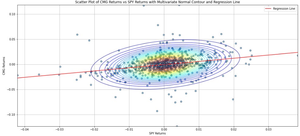
Note that if we draw a 2D Gaussian contour over the data, the line of best fit would intercept the layers of the contour at points where it is perpendicular to the vertical tangent of the contour. This is since the line of best fit minimizes the (squared) distance from the data, so that at any point the distance between the line of best fit and the top and bottom of the contour must be the same. As such, the line of best fit must be perpendicular to the vertical tangent when it exits the contour.

Using the same reasoning, the line of best fit of the regression in the inverse direction must go through the points on the contour where the tangent is horizontal instead of vertical. As such, the two lines would not be reciprocals of each other unless the contour was a straight line i.e. R2 = 1. In fact, by inspecting the formulas for the two betas (form SPY to CMG and from CMG to SPY), we note that the product of the betas is R2. When there is no causality between the variables (i.e. contour is a circle) then the lines of best fit are perpendicular to each other and the R2 approaches 0.

In our case, the beta when SPY is the predictor is 0.63 and the beta when CMG is the predictor is 0.12, which is less than the reciprocal of 0.63. This suggests that SPY returns are much more informative of CMG returns than CMG returns are of SPY returns, which accords with our intuition. This is partially what points (1) and (2) mean when we say that regression is all about causality and how one variable impacts another. Of course, spurious correlations can and do often happen. Mathematics is a tool that we should use with caution and reason, rather than blindly apply.

Disclaimer

The information provided on TheLogbook (the "Substack") is strictly for informational and educational purposes only and should not be considered as investment or financial advice. The author is not a licensed financial advisor or tax professional and is not offering any professional services through this Substack. Investing in financial markets involves substantial risk, including possible loss of principal. Past performance is not indicative of future results. The author makes no representations or warranties about the completeness, accuracy, reliability, suitability, or availability of the information provided.

This Substack may contain links to external websites not affiliated with the author, and the accuracy of information on these sites is not guaranteed. Nothing contained in this Substack constitutes a solicitation, recommendation, endorsement, or offer to buy or sell any securities or other financial instruments. Always seek the advice of a qualified financial advisor before making any investment decisions.