Why Betting Markets Move Differently Compared to Polls & Models

How uncertainty in an event actually reduced the volatility of its probability over time

True probabilities must be martingales over time (directionally unpredictable) because if they were not, a trader could construct a strategy that is positive expectancy, showing that the traded odds were not on average fair. In addition, the evolution of an event contract’s price over time must obey arbitrage constraints regarding their volatility; since probabilities are bounded between 0 and 1, their diffusion must respect absorbing barriers, which manifests in a volatility limit that scales with the uncertainty of the probability estimate itself. In this post we draw upon papers and tweets posted in the Taleb-Silver Twitter War.

Treating Probabilities as Financial Instruments

A martingale process is a stochastic (i.e. has elements of randomness) process in which the conditional expectation of the next value, given all past information, is equal to the current value. In the context of probabilities or betting odds, this means that the “correct” expected future probability of an event remains equal to its present probability, preventing any systematic patterns that could be exploited.

If odds are "true" in the sense that they correctly reflect the real-world probabilities of outcomes, then by the linearity of expectation, any wager placed on them cannot have a negative expected value. Since true odds are also tradable odds (i.e., they can be bet on in a market setting), they must satisfy no-arbitrage constraints, which impose conditions on their evolution (more details later).

We claim also that as the volatility of a symmetrically distributed underlying asset increases, arbitrage forces push the forward price of a corresponding binary option (a financial derivative that pays a fixed amount, say 1, if the asset is above a certain price at expiry and nothing otherwise) toward 0.5 and reduce the option’s own volatility over time. This occurs because increased uncertainty in the underlying makes the probability of being above the barrier more balanced between occurring and not occurring, reducing the ability to confidently assign extreme probabilities. In other words, counterintuitively, higher uncertainty about the underlying asset leads to a lower volatility in the binary option price.

This principle should apply universally in any domain where binary prices are produced, including probabilistic forecasting of events like elections or sports (although it is difficult here to define what the “underlying” is; maybe expected difference of votes / scores). However, empirical observations show significant violations of these principles, particularly in the 2016 U.S. presidential election where some predictors gave the candidate Donald Trump between 1% to 30% chance of success and had jumps in the revisions of forecasts from 50% to 10%. For example, Nate Silver’s prediction in 2016 exhibits a high degree of volatility

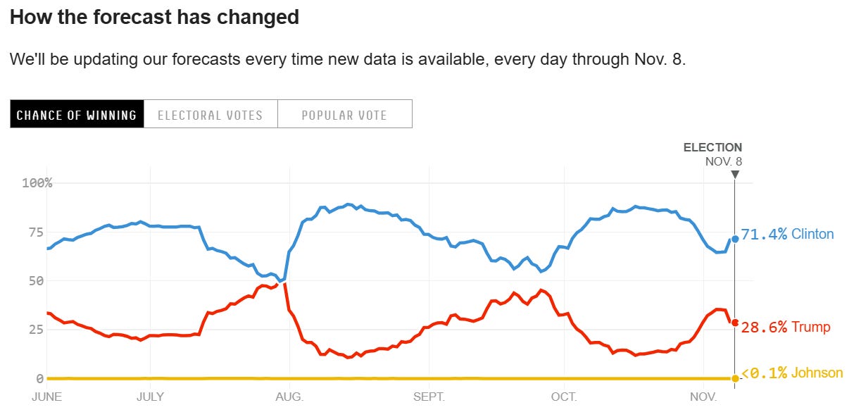
While much has been written about why polls got it wrong in 2016, this post isn’t about the lessons that pollsters learned after the elections, but rather why naively using polling data (or indeed, any other non-martingale process) to construct probabilities (which we noted ought to be martingale over time) is problematic. In particular, we note the following points

1. Probabilities can’t be constructed with only functions of non-martingale inputs

2. Increasing uncertainty in the “underlying event” should decrease the volatility of the event contract associated with the event over time and push it towards 50%

3. It is possible to produce no-arbitrage probabilities over time using a local volatility model for the instantaneous returns of the binary option

4. Probabilities as martingales is consistent with Bayesian updating framework

Probabilities can’t be constructed with only functions of non-martingale inputs

Probabilities cannot be constructed using only functions of non-martingales because any deterministic transformation of a non-martingale will generally inherit its predictability, violating the fundamental property that a probability forecast should not exhibit arbitrageable trends. In the context of election forecasting, consider how polling averages often experience predictable upticks following key campaign events such as party conventions or vice-presidential nominations.

If a probability forecast were constructed solely as a function of raw polling data, it would inherit this predictable drift, meaning the forecast would systematically increase post-convention—even when no new, unexpected information about the election outcome has emerged. This violates the martingale property, where the best estimate of future probability should be today’s probability, adjusted only by unexpected new information. Instead, a well-calibrated probability forecast must incorporate the expected drift in polls, meaning it should already account for the anticipated post-convention bump. The probability should only update when the realized movement in polling differs from the expected effect—ensuring that the forecast remains a proper martingale and does not allow for arbitrage-based trading strategies that profit from predictable mispricing.

Increasing uncertainty in the “underlying event” should decrease the volatility of the event contract associated with the event over time and push it towards 50%

The main results of this section are drawn from the paper “Election Predictions as Martingales: An Arbitrage Approach” by Taleb and “All roads lead to quantitative finance” by Taleb & Madeka. The paper explores how we can define the forecasted probability as a function of the observed vote share at the time such that the prediction is arbitrage-free. The paper uses the following definitions

Y0 is the observed estimated proportion of votes expressed in [0, 1] at time t0. These can be either popular or electoral votes, so long as one treats them with consistency. T is the time when the irrevocable final election outcome YT is revealed, or expiration. t0 is the present, hence T −t0 is the time until the final election, expressed in years. s is the annualized volatility of Y, or uncertainty attending outcomes for Y in the remaining time until expiration. We assume s is constant without any loss of generality –but it could be time dependent. B(.) is the "forecast probability", or estimated continuous time evaluation of the election results, which can be used to establish arbitrage bounds between B(.), Y0 and the volatility s.

The main result of the paper (not that important for intuition) is that

\(\begin{equation} B(Y_0, \sigma, t_0, T) = \frac{1}{2} \operatorname{erfc} \left(\frac{l - \operatorname{erf}^{-1} (2Y_0 - 1) e^{\sigma^2 (T - t_0)} }{\sqrt{e^{2\sigma^2 (T - t_0)} - 1}} \right), \end{equation}\)

Where l is the proportion of votes needed to win (0.5 typically) and erfc is the standard complementary error function, given by

\(\operatorname{erfc}(z) = 1 - \operatorname{erf}(z), \ \ \ \ \ \operatorname{erf}(z) = \frac{2}{\sqrt{\pi}} \int_0^z e^{-t^2} dt\)

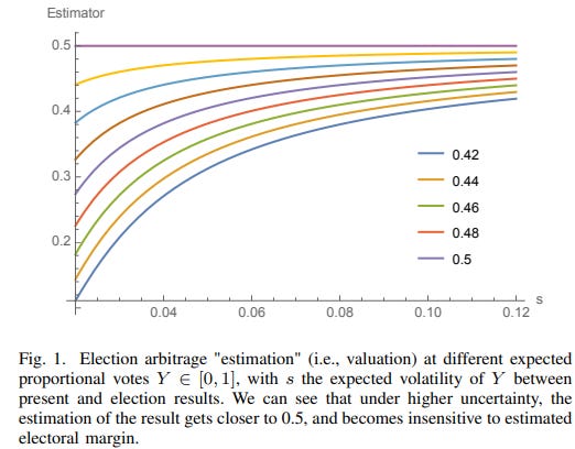
The proof of the above result is outside the scope of this post, but we can see that according to the result given, that as the volatility of the “underlying process” corresponding to the event contract (to the time to expiry) approaches infinity, we can show (with some messy math) that the probability should approach 0.5.

Intuitively, if the vote share is modeled as a bounded arithmetic Brownian motion then over an infinite time horizon with nonzero volatility (or vice versa), it can theoretically end up on either extreme with roughly equal probability, regardless of initial conditions (and therefore push the value of the event contract to 1/2).

It is also interesting to consider why arbitrage is possible if the volatility of the probability given by the forecaster is too high. In particular, if the probability forecast jumps up and down excessively, a simple buy low, sell high strategy can be used to generate a profit. To formalize this, let the forecast probability B(t) evolve according to the SDE (where W(t) is the Wiener Process)

\(dB_t = \sigma dW_t,\)

Now consider a simple trading strategy that buys when B(t) is too low (relative to B0​) and sells when B(t)​ is too high, in proportion to the difference. Its PnL is represented by the stochastic integral

\(\int_0^T (B_0 - B_t) dB_t = \frac{1}{2} \sigma^2T - \frac{1}{2}(B_T - B_0)^2\)

The integral is solved via a direct application of Itô's lemma, which is outside the scope of this post. Intuitively, since the right-hand side is always nonnegative (due to the squared term), the strategy suggests that if B(t) is too volatile, then an arbitrage opportunity exists (assuming constant volatility over time). As such, even when the underlying process (polled vote share) may experience wide variations, the actual probability traded shouldn’t (see visualization below):

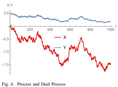
The exact bound for the volatility of the estimator doesn’t have a closed-form solution, but Taleb provided a numerical visualization in his paper:

It is possible to produce no-arbitrage probabilities over time using a local volatility model for the instantaneous returns of the binary option

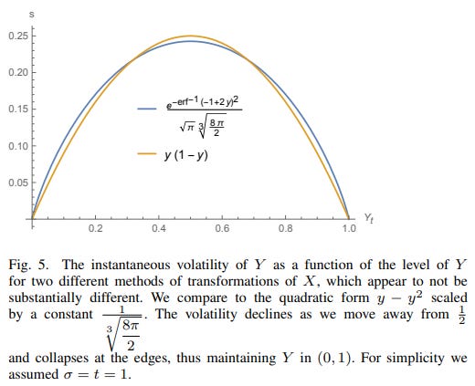
It is possible to construct no-arbitrage probabilities over time by modeling the instantaneous returns of the binary option using a local volatility model. This approach recognizes that part of what it means for a probability to be well-calibrated—whether high or low—is that its fluctuations over time must be constrained (i.e. greater confidence necessarily means less uncertainty).

For example, if an event is assigned a 90% probability, then under a correct probabilistic framework, it should only cross over to the opposite outcome exactly 10% of the time. Similarly, if the probability is 99%, it should only reverse course 1% of the time. This constraint inherently reduces the volatility of probabilities as they move toward extreme values, preventing large, unjustified swings.

This aligns with intuition: if an event is overwhelmingly likely, its probability should not exhibit excessive fluctuations. Thus, a properly constructed probability process must incorporate this volatility suppression effect, ensuring that extreme probabilities remain stable (once we’ve reached / near them) while intermediate probabilities remain more responsive to new information (and therefore can have greater vol).

Probabilities as martingales are consistent with Bayesian updating framework

Martingale pricing is naturally compatible with Bayesian updating because both frameworks rely on the idea that future expectations should be fully incorporated into present values. In Bayesian updating, a forecast probability represents our best estimate given all available information, and when new data arrives, we update our beliefs in a way that remains internally consistent with prior probabilities and expected changes. Similarly, in a martingale framework, the current probability must already reflect the expected value of future probabilities, meaning that the best forecast of tomorrow’s forecast is today’s forecast itself.

This connection becomes clear in election forecasting. Suppose we are estimating a candidate’s probability of winning the election. If we expect the probability to shift upward over time due to predictable factors (such as economic improvement or campaign momentum), then that expected shift should already be included in today’s probability. If not, we are systematically underestimating the candidate’s chances. Bayesian updating naturally enforces this by requiring that today’s probability integrates all prior knowledge about how the election might evolve. In other words, if we could anticipate that a probability will change in a certain direction, then Bayesian reasoning dictates that it should already have changed in that direction—just as in a martingale pricing framework, where the expected value of an asset at a future time is simply its current value under the risk-neutral measure.

A direct implication of this is that probability movements should be constrained based on their starting values. If a forecast assigns a 90% probability today, then by definition, the probability should only cross to the other side 10% of the time. If it is at 99%, it should only flip in 1% of cases. This aligns with Bayesian reasoning: the degree of confidence in a forecast must correspond to the likelihood of extreme updates. If a probability moves too much in predictable ways, it suggests that the model was initially miscalibrated—either underestimating or overestimating uncertainty.

Pollsters and Prediction Markets are Talking About Different Things

Pollsters and prediction markets are often mistaken as providing the same type of information, but in reality, they are answering very different questions. Pollsters estimate the probability of a candidate winning if the election were held today, while prediction markets aim to estimate the actual probability of a candidate winning in the future, incorporating all expected developments between now and Election Day. This fundamental distinction explains why polls and market prices can diverge significantly in the months leading up to an election.

Polls are snapshots of current public opinion, reflecting the preferences of surveyed voters at a given moment. A poll showing a candidate ahead by five points today does not imply that the candidate will maintain that lead weeks or months later. In contrast, prediction markets attempt to price in all future uncertainty by factoring in expected campaign developments, voter decision shifts, and external shocks. Market participants are not just reacting to today's polls but also to their own expectations of how sentiment will evolve and how much uncertainty there actually is.

Because of this difference, polls and prediction markets should converge as Election Day approaches, but their behavior along the way will differ significantly. Early in the campaign, markets should move much less than polls, as traders recognize that individual polling swings are often noise and do not necessarily reflect lasting changes in voter sentiment. Markets remain relatively stable because they price in the likelihood of reversion to long-term fundamentals, such as partisanship, economic conditions, and historical election patterns.

However, as the election nears, markets may become more volatile than polls, especially in response to major late-breaking developments such as scandals, economic surprises, or turnout shocks. This is because as uncertainty about the future resolves, market participants will adjust their expectations sharply. For example, if polls show a close race leading up to Election Day, but markets believe that one candidate has a structural advantage in mobilization or late-deciding voters, markets may swing more than the final round of polling. Similarly, if unexpected results begin emerging on Election Night, markets will react instantly.

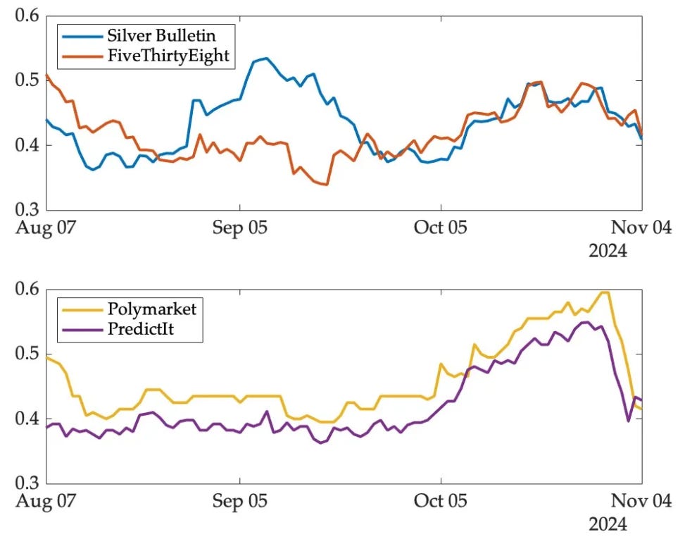
For example, the figure below shows the probability assigned to a Trump victory in Wisconsin (2024) by two pollsters (top panel) and two markets (bottom panel) over the ninety days leading up to the election:

The General Lesson About Event Forecasting

This distinction between polls and prediction markets applies broadly to all types of event forecasting, including financial modeling and sports betting. In every case, there is a fundamental difference between models that reflect current conditions and those that attempt to estimate the true probability of the final outcome by incorporating future uncertainty.

In sports betting, for example, power rankings, team statistics, and expert analysis serve a similar role to polls in election forecasting—they measure a team's current strength based on past performance and immediate conditions. However, betting markets do not simply price in who is the best team today; they attempt to anticipate how the season will unfold, incorporating factors like injuries, upcoming schedule difficulty, player development, and potential coaching adjustments. A team with a dominant early-season record may still have relatively long championship odds if markets expect them to regress or face tougher competition later on. Similarly, a struggling but highly talented team may have more favorable odds than their current record suggests because markets expect them to improve.

The same logic applies to financial markets and event contracts. In finance, a company’s stock price does not reflect its current profitability alone—it prices in expectations of future earnings, economic conditions, and industry trends. If a company beats earnings estimates today but provides weak future guidance, its stock may drop despite strong present performance. Just like political prediction markets, financial markets smooth out day-to-day volatility and only make large adjustments when truly new information emerges that alters long-term expectations.

In event contracts—such as those on platforms like Kalshi, where traders bet on outcomes like interest rate hikes, climate events, or geopolitical developments—the same principles hold. A contract predicting whether inflation will exceed 3% by the end of the year will not simply reflect the current inflation rate; instead, it will incorporate market expectations of future economic trends, central bank policy shifts, and external shocks. A sudden rise in inflation today might not cause the contract to surge if traders believe it is temporary, just as a candidate’s strong poll today might not meaningfully shift their prediction market odds if traders expect the race to tighten.

Across all these domains, the core principle remains the same: models and forecasts that focus on current conditions are distinct from markets and betting odds that price in future uncertainty. The two should converge as the event approaches because, eventually, there is no more uncertainty left to incorporate. But at earlier stages, markets tend to move more cautiously than models that focus only on the present. Understanding this distinction helps explain why betting markets, financial markets, and political prediction markets often seem slow to react to short-term developments—while also allowing them to make sharper adjustments when the event is truly imminent.

Disclaimer

The information provided on TheLogbook (the "Substack") is strictly for informational and educational purposes only and should not be considered as investment or financial advice. The author is not a licensed financial advisor or tax professional and is not offering any professional services through this Substack. Investing in financial markets involves substantial risk, including possible loss of principal. Past performance is not indicative of future results. The author makes no representations or warranties about the completeness, accuracy, reliability, suitability, or availability of the information provided.

This Substack may contain links to external websites not affiliated with the author, and the accuracy of information on these sites is not guaranteed. Nothing contained in this Substack constitutes a solicitation, recommendation, endorsement, or offer to buy or sell any securities or other financial instruments. Always seek the advice of a qualified financial advisor before making any investment decisions.