Decomposing Volatility Skew

A Linear Factor Extension of Local Volatility

When we talk about the skew of a single stock, we usually treat it as a single, unified thing. That story is true in the average case, and it is a perfectly serviceable first model. But it papers over something important. A single stock is not a single exposure. It is a basket of exposures stacked on top of each other: exposure to the broad market, exposure to its sector, exposure to its industry, and a residual exposure that is the stock’s idiosyncratic “self.” Each of these has its own relationship with volatility. On any given period, the move you observe in the stock can be driven by any one of them, or any combination, and the vol response can swing accordingly.

What is Volatility Skew

Briefly, the implied volatility of an option is the volatility you would have to plug into Black-Scholes to make the model price match the observed market price. Different strikes on the same expiry generally trade at different implied vols, and a plot of implied vol against strike is called the volatility skew (or smile, or smirk, depending on its shape). For equity indices and most single names, the curve slopes down, downside puts trade at higher implied vols than upside calls, which is what practitioners mean when they say “equity skew is negative / put-skewed.”

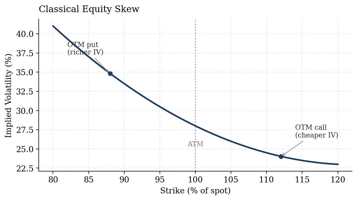
Where does that asymmetry come from? The classical answer is spot-vol correlation.

If realized volatility tends to rise when the spot falls, which it overwhelmingly does in equities, then the paths that finish below an OTM put’s strike are paths along which vol has on average been higher than usual, so the strike vol on the put has to compensate and prints rich.

Symmetrically, the paths that finish above an OTM call’s strike are paths along which vol has been compressing, and the strike vol on the call prints cheap. This is the dynamic, or local-volatility, view of skew: skew exists because the underlying’s vol moves opposite to its price.

So far, so standard. The thing the standard story leaves implicit is that “the underlying’s vol moves opposite to its price” is an empirical statement about a single, undifferentiated random variable: the stock. The stock, however, is not a primitive variable. It is a function of underlying drivers, and the vol response to those drivers does not have to point in the same direction.

Decomposing the Stock

When we talk about a stock’s daily P&L, we are perfectly comfortable saying “today NVDA was up three percent, but index was up two so that was expected.” That is a casual decomposition of return into a market-beta component and an idiosyncratic component. We do not think of the stock’s daily return as a primitive; we routinely partition it.

What naturally follows is that we ought to partition is the stock’s vol response to those moves. A naive local vol model treats spot-vol correlation as a single function of the single variable “stock price.” But if the return can be decomposed into a beta piece and an idio piece, the spot-vol relationship can be decomposed too. The vol of the stock responds differently to a one percent move that is the index’s fault than it does to a one percent move that is purely the name’s own, and those two responses, importantly, can point in opposite directions.

Consider a meme stock with a beta to the broad market, sitting in some otherwise normal macro regime. Hold all else equal and consider each of the following moves.

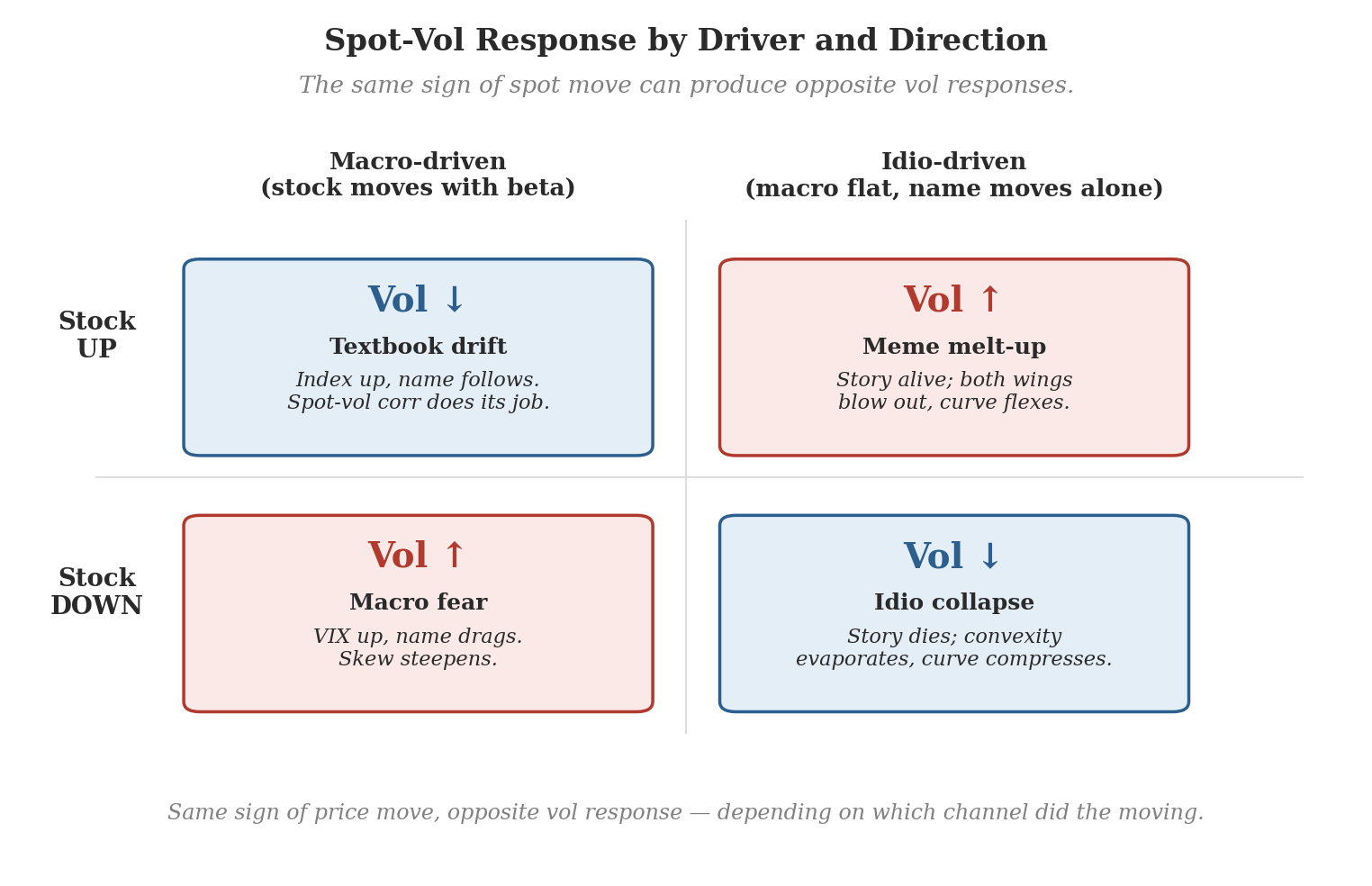
Case 1) Stock up with beta, slow and orderly. The S&P drifts up half a percent over the morning, the stock follows it up about a percent in line with its beta, nothing unusual is happening. Implied vols on the index and the stock decline modestly.

Case 2) Stock up violently, while the market is flat. The vol response here is positive. The meme is signaling that it has not yet died, and option markets respond by paying up for upside.

Case 3) Stock down with the market. The S&P sells off two percent on a macro headline; the stock sells off three in line with beta. Here we are back in the textbook. Vol goes up. VIX goes up. Skew steepens.

Case 4) Stock down, while the market is flat. This is the case that most clearly exposes the limits of the single-factor view. The market is fine. The stock idio drops ten percent as the meme deflates into nothing. The vol response here is negative. The story is over. The convexity is gone. Forward realized vol on the name collapses because the source of variance itself (the meme) has evaporated.

Two Skews, One Curve

The same sign of spot move gives the opposite vol response depending on whether the move was macro-driven or idio-driven. The realized correlation between the stock’s price and its vol is therefore not a single number but a blend of two underlying numbers, with the weights set by which channel is currently doing the moving.

If we adopt the local-volatility view that skew is the option market’s pricing of spot-vol correlation, then the skew on a single name must, by the same logic, be a blend of two skew curves:

• A macro skew, inherited from the stock’s beta exposure to the broad market. This is the equity-fear curve with negative spot-vol correlation, OTM puts richer than OTM calls, the classic SPX-style smirk on a smaller scale.

• An idio skew, reflecting the stock’s spot-vol relationship at the residual level. The shape of this curve depends on what the name actually is.

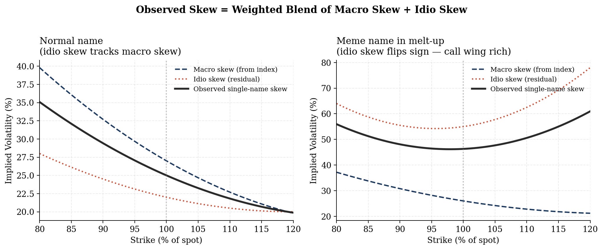
The skew you observe on the option chain is some weighted combination of those two underlying curves, weighted by roughly the relative contribution of macro and idio variance to the name’s total variance (technically not true since the macro skew also takes into account the correlation between spot and index-wide correlation but for the purposes of this post let us not consider additional effects).

This isn’t strictly additive. Spot-vol relationships aren’t linear; beta itself isn’t constant; and the conditional distribution of an idio move given a macro move is messy. The decomposition is best read as a heuristic, not an identity.

Further Decompositions

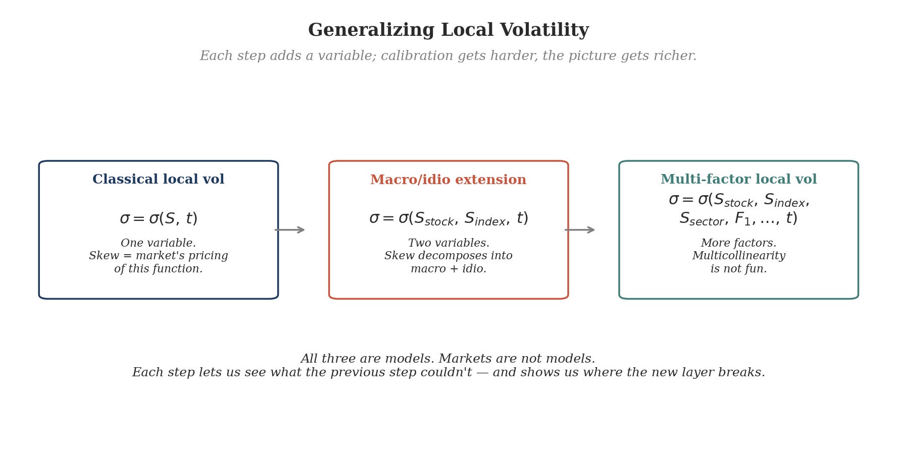
Classical local volatility writes the instantaneous vol of an asset as a function of its own spot price and time, σ = σ(S, t). The observed skew curve is the option market’s pricing of that function.

What we have just argued is that, for a single stock, the relevant local-vol function isn’t really σ(S_stock, t). It is closer to σ(S_stock, S_index, t) with two variables. And there is no principled reason to stop at two. You could extend to σ(S_stock, S_index, S_sector, t), or further.

A name in semis might want a separate factor for AI Capex. A bank might want a rates factor and a credit spread. A miner might want the commodity. Each new variable opens another channel through which spot moves can be sourced and through which vol can respond differently.

However, there is a calibration asymmetry that makes the macro/idio decomposition especially useful. We have deep, liquid options markets on the broad index such as SPX, NDX, and RUT. The macro skew is therefore directly observable. We can pull a clean macro spot-vol relationship off market prices any trading day of the week. We do not, in general, have clean factor option markets for the things that drive other aspects of vol.

But when we do, a linear multi-factor local vol model is the simplest possible generalization of single-asset local vol. Though as soon as we permit ourselves to do this, the usual problems of any multi-factor linear model show up as the inputs are correlated with each other, the loadings shift across regimes, and calibration is underdetermined.

You could also put flow into the model. You could put dealer options-positioning. You could put a sentiment index or a search-trend metric also. Each of those will, in principle, shift the conditional vol of a single name. The macro/idio decomposition is just the cleanest two-factor approximation to a much higher-dimensional problem; we pick it because we can always see the macro piece in liquid index options, not because it is the only piece that matters.

Closing Thoughts

None of what we’ve written here is a description of reality. Markets are not models. Markets are what models try to explain, and any model elegant enough to be useful is going to be wrong in interesting places. However, at times each new layer of does give us a sharper articulation of what the market is currently pricing, and by contrast it shows us the places where the market is doing something we don’t yet accommodate.

The places the model breaks are the places that matter, because those are the places where the market is telling us something we did not yet have a word for. When that happens, and it happens often, we get to make better models (and make a lot of money along the way). The two-skew view is one such step. There are many more.

Disclaimer

The information provided on TheLogbook (the “Substack”) is strictly for informational and educational purposes only and should not be considered as investment or financial advice. The author is not a licensed financial advisor or tax professional and is not offering any professional services through this Substack. Investing in financial markets involves substantial risk, including possible loss of principal. Past performance is not indicative of future results. The author makes no representations or warranties about the completeness, accuracy, reliability, suitability, or availability of the information provided.

This Substack may contain links to external websites not affiliated with the author, and the accuracy of information on these sites is not guaranteed. Nothing contained in this Substack constitutes a solicitation, recommendation, endorsement, or offer to buy or sell any securities or other financial instruments. Always seek the advice of a qualified financial advisor before making any investment decisions.